• Introduction
• DBNs
• Structure learning for DBNs
• Implementation

The code for this demo can be found here.

Introduction

We saw earlier how Bayesian Networks can be used to create a probabilistic model of a dataset, and how it can represent independence assumptions between each variable. In this post we’ll talk about how we can extend this framework to account for temporal effects, such as modelling time series.

DBNs

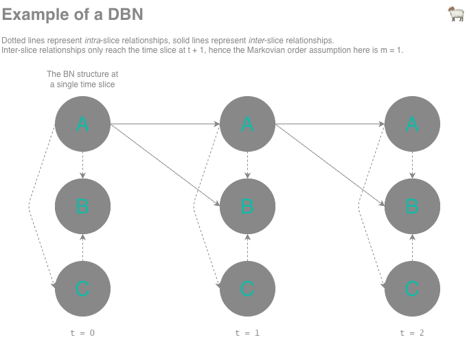
Bayesian Networks are a powerful tool for representing causal and dependence relationships between variables, but they can also model how variables evolve over time. The Dynamic Bayesian Network (DBN) extends BNs to do this by discretising time into slices¹, where:

• Each slice contains its own Bayesian Network, these are called intra-slice BNs and their structure is fixed across time (although there do exist time-varying Bayesian Networks where the BN can vary over time).
• Variables in one slice can influence variables in future slices, referred to as inter-slice relationships.
  • No variable is allowed to affect variables in a past time slice.

Formally, DBNs are represented as follows. Recall that the joint probability distribution of Bayesian Networks may be represented like this:

Where $x_i$ represents node/variable $i$, and $\mathbf{Pa}_i$ represents the parents of node $i$.

To account for time $T$, every BN slice needs to depend on the BN slices that came before it temporally - so the joint probability becomes this:

Where $\mathbf{X}^t = \{X_1^t, \ldots, X_n^t\}$ represents the set of nodes in time slice $t$.

However, this gets unwieldy as the number of time slices we need to account for increases. In order to keep the problem tractable, a Markovian order assumption is often introduced. Here, we stipulate that a time slice is independent of any slices that are $m$ steps prior - where often $m=1$, which simplifies the joint probability down to:

Structure learning for DBNs

We’ve already talked about using hill-climbing for structure learning in Bayesian Networks, we can also use hill-climbing to learn the structure of DBNs. The dbnR package makes use of dynamic hill-climbing, which:

• Performs an intra-slice pass, learning the relationships between variables within a given time slice. This is essentially a regular BN structure learning problem.
• Then performs an inter-slice pass, learning how variables in $t-1, t-2, …, t-m$ affect variables in $t$ (the current time slice).
  • The blacklist argument of bnlearn::hc() is utilised here to ensure that no future → past relationships are learned.

These two structures are then combined to form the final DBN.

Implementation

In this demonstration, we’ll be predicting the rate of Influenza-Like Illnesses (ILI) across the United States’ 10 Health and Human Services (HHS) regions. DBNs work well in this example since the ILI rate is less severely autoregressive than series such as stock data, and each variable has a genuine causal link to other variables (through the geographical spread of flu-like illnesses).

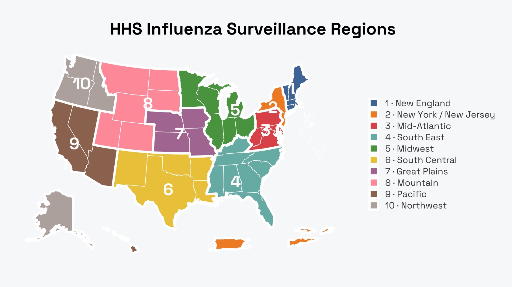
The first thing we’ll need is the data. We’ll use the cdcfluview package to source this. Then, since we want each HHS region’s ILI rate as a variable, we’ll pivot this table to wide format.

flu_raw <- cdcfluview::ilinet(region = "hhs", years = 2010:2019)
 
flu_wide <- flu_raw %>%
  select(week_start, region, weighted_ili) %>%
  mutate(region = str_replace(region, '^Region\\s', 'hhs') %>% tolower()) %>%
  pivot_wider(names_from = region, values_from = weighted_ili) %>%
  arrange(week_start) %>%
  filter(if_all(starts_with("hhs"), ~ !is.na(.x)))

From here, we can calculate the change in ILI rate over time in each HHS region, then split the dataset up into 80% train and 20% test. We then learn the DBN structure of the data, then the parameters of the network:

# Structure learning first, then fit parameters using MLE-Gaussian
net  <- dbnR::learn_dbn_struc(train, m)
size <- attr(net, "size")
fit  <- dbnR::fit_dbn_params(net, dbnR::fold_dt(train, size), method = "mle-g")

We can visualise what structure the DBN has learnt by running plot(fit):

Upon inspection of this structure, we can start to learn a few things about the data. For example:

• HHS6 depends on HHS7 within each slice. We can’t say that HHS6 is caused by HHS7 here, but we can say that they tend to move together over time.
• HHS8 depends on HHS7 from the previous slice. We can take this as a 1-week predictive lead, i.e. HHS8 tends to increase in infection the week after HHS7 starts increasing.

Finally, we can predict a 1-step rolling forecast using this fit and dbnR::forecast_ts. Recall that we are initially predicting the week-on-week change to avoid a rank-deficient covariance matrix:

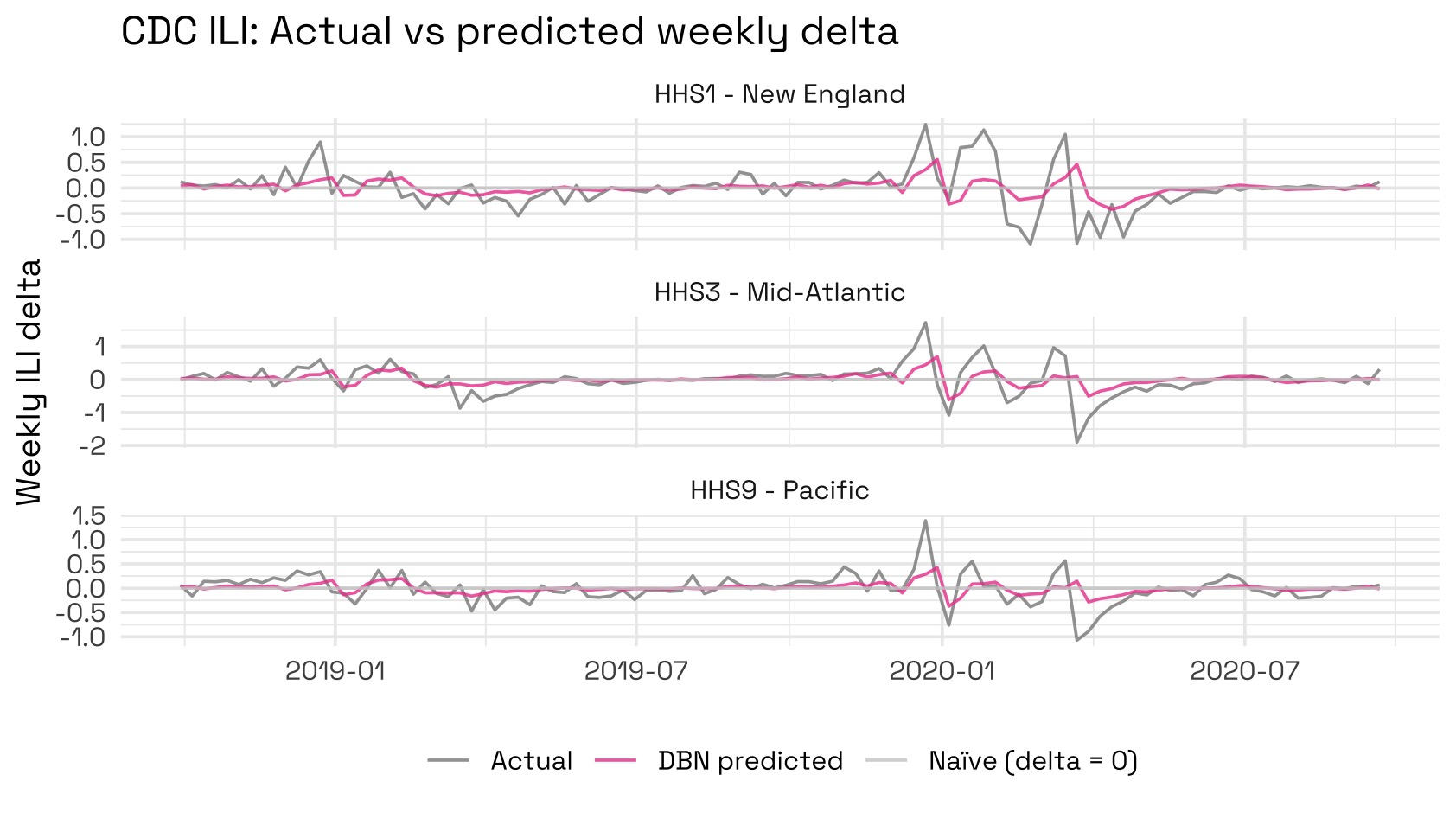
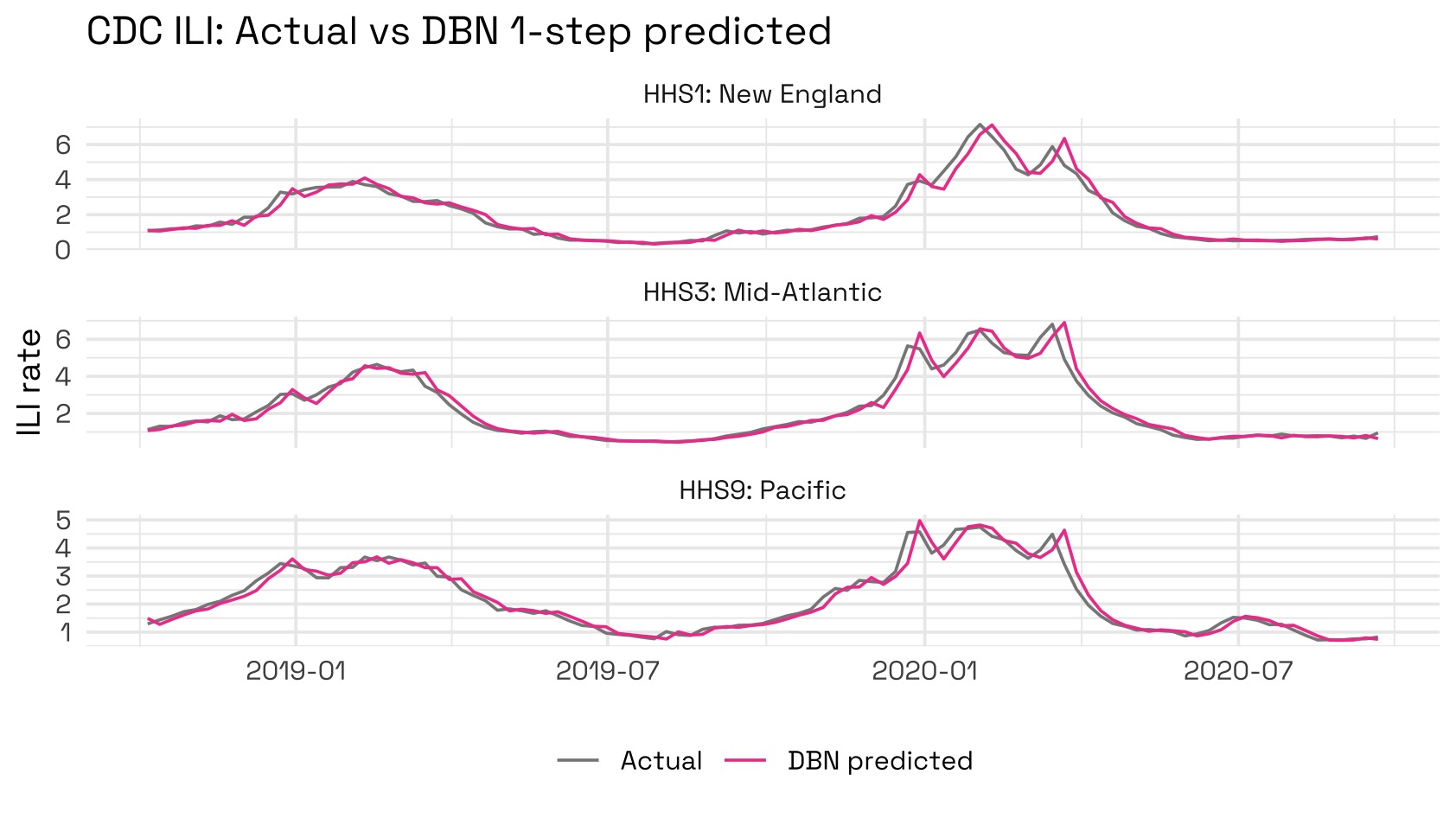
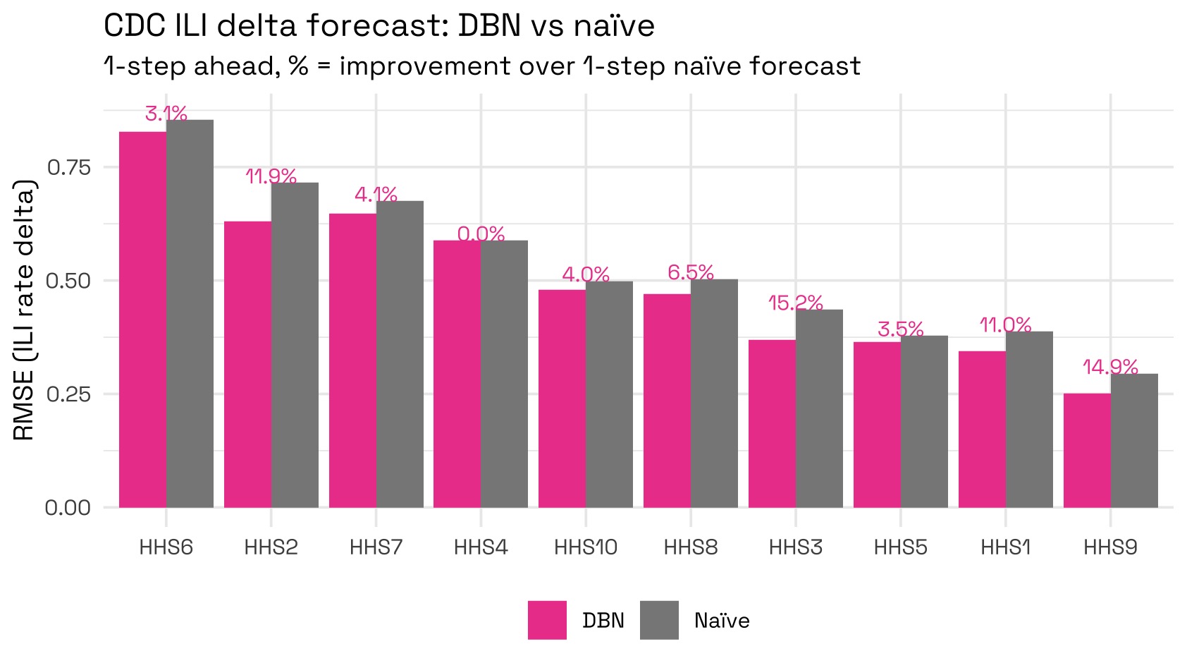
We can see that the model generally seems hesitant to predict large changes from the last week due to its Gaussian nature; however it does beat the naïve forecast strategy of predicting 0 changes. To quantify how much better the DBN does compared to the 1-step naïve forecast strategy, we can visualise each method’s RMSE:

We can reconstruct forecast levels and compare them against actuals to see that in general, the forecasts do quite well.