- Published on
- • 14 min read
Structure Learning in Bayesian Networks
- Authors

- Name
- Darren Wong
- Socials
- Darren's site
The code for this demo can be found here.
Introduction
Bayesian Networks (BNs) are a tool for building a probabilistic model of a dataset, providing a way to encode prior knowledge in the process. BNs are directed acyclic graphs (DAGs) that represent independence assumptions amongst variables. Their key property is that a variable is independent of all other variables that don't descend from it, once you know the values of its parents. Unlike many modelling approaches, BNs are highly interpretable: the graph itself is the explanation, showing explicitly how each variable influences the others.
With this graph in hand, we can infer conditional and marginal independence properties as well as results of other probability operations through graph manipulations. We can also perform what-if reasoning, e.g. if I observe high Glucose, what does that tell me about the probability of someone having Diabetes?
Beyond inference, BNs are a Bayesian construct: they represent variables as probability distributions rather than point estimates. This means the model carries uncertainty through every variable, which is useful in fields such as medicine and science where uncertainty quantification matters. This also means that we can incorporate prior knowledge directly into the structure or parameters, rather than letting the data speak entirely on its own.
Motivation
Say we have data with binary variables . The joint distribution is ; but to specify all possible combinations of each variable in a joint probability table, we’d need rows, e.g. for the joint probability of tossing three coins we’d have 8 rows:
| H | H | H | 1/8 |
| H | H | T | 1/8 |
| H | T | H | 1/8 |
| H | T | T | 1/8 |
| T | H | H | 1/8 |
| T | H | T | 1/8 |
| T | T | H | 1/8 |
| T | T | T | 1/8 |
Performing inference like computing the marginal distribution of would then require summing over states of the other variables. This quickly becomes intractable as increases in size.
To handle this, we need to constrain the nature of variable interactions. The primary feature of BNs is factorisation of the joint probability distribution. Here’s how it works:
First, we use the probability chain rule to break the joint distribution down into smaller terms:
This alone is not entirely useful, we’ve created three tables, the largest of which still requires space to represent. Note that we can place the variables in any order in the chain rule and it’d be equivalent, however some orderings are more useful than others.
Number of parameters required to specify an unfactorised joint distribution
Technically, the number of parameters it takes to represent an unfactorised probability distribution is . Here that’d be .
The truly useful bit is if we were clever enough to order variables in the chain rule so that causes come before effects. That way, we can use our domain knowledge to knock out variables from each conditional probability term. Say for example that we know is a root cause for and . That means that the value of wouldn’t depend on the value of or , so this term is equivalent to . The joint probability distribution is now:
This now requires parameters to specify. For a dataset with large , the savings are substantial, and they compound quickly since each additional parent you give a node multiplies the number of parameters it needs (so it grows exponentially).
Number of parameters required to specify a factorised joint distribution
The number of parameters it takes to represent a factorised probability distribution is . Here that’s .
Now we’re cooking with gas.
Structure learning
There are two main components we need to define a Bayesian Network over our data:
- The structure, i.e. the graph and all the independence assumptions that come along with it; and,
- The parameters which are essentially the conditional probability tables derived from the data.
We’ll focus on learning the structure in this post. There are a few ways of doing this but we’ll focus on the score-based method since this seems to be a more robust way of learning the structure of a graph. Score-based structure learning treats the graph learning task as an optimisation problem, and the specific algorithm we’ll be using is greedy hill-climbing (HC). How it works is as follows:
- Start with a given network (an empty graph or one built using prior knowledge). Each iteration:
- Check the score for all possible graph mutations (adding an edge between two nodes, deleting an edge between two nodes, or reversing the direction of an existing edge)
- Choose the action that provides the highest score gain (the greedy part of this algorithm)
Like most greedy algorithms, hill-climbing does sometimes get stuck in local maxima or plateaus. Random restarts help with both of these issues. Further, Tabu Search is an add-on to hill-climbing that forbids recently visited moves, which helps the HC algorithm avoid getting stuck in local optima.
But how do we define the ‘score’ in this case?
The score function
There are many different score functions we can use, but the common threads amongst most of them are:
- They measure the strength of the relationship between a node and its proposed parents in some way.
- They are score equivalent, which in a nutshell means they produce the same score over graphs that encode the same independence assumptions.
- They are decomposable which means that we can decompose the score of a network into the sum of the scores of the individual nodes (which helps a lot for parallel processing and for quickly assessing the score impact of different graph mutations).
- The ones that generally perform the best are regularised which means they penalise more complex graph structures in favour of simpler ones.
The score function we’ll use in this demo is the Bayesian Information Criterion (BIC) which meets all of the above criteria. Let’s break this down.
Formally, the BIC is defined as:
- is the number of samples in our dataset
- is the sum of the mutual information between node and its parents for all nodes.
- What this really measures is how much information does knowing the parents of tell you about itself? The higher this value, the stronger the mutual information, and the stronger the dependency is.
- is the sum of the entropy of each node, we consider this a constant, so we are really trying to maximise here.
- is our regulariser. It’s the log of the number of samples in our dataset multiplied by the number of independent parameters in .
In summary, this measures how strong the dependency of each node is on its parents, which is tempered by the regularisation term which grows larger the more edges there are in the graph. It is important to note, however, that grows linearly as increases - but the regularisation term grows logarithmically. What this means is that as grows larger, this function is happier to accept more complex models, since there is enough data to back those relationships up.
Note
As , the BIC approaches the Bayesian score which uses a prior over the graph structure to control graph complexity.
R Implementation
We’ll be running the hill-climbing algorithm over the Pima Indians Diabetes database, which aims to predict whether or not a patient has diabetes based on certain diagnostic measurements. We’ll use RKaggle to avoid fumbling around with CSV files:
diabetes <- RKaggle::get_dataset('uciml/pima-indians-diabetes-database')

glimpse(diabetes)
#> Rows: 768
#> Columns: 9
#> $ Pregnancies              <dbl> 6, 1, 8, 1, 0, 5, 3, 10, 2, 8, 4, 10, 10, 1…
#> $ Glucose                  <dbl> 148, 85, 183, 89, 137, 116, 78, 115, 197, 1…
#> $ BloodPressure            <dbl> 72, 66, 64, 66, 40, 74, 50, 0, 70, 96, 92, …
#> $ SkinThickness            <dbl> 35, 29, 0, 23, 35, 0, 32, 0, 45, 0, 0, 0, 0…
#> $ Insulin                  <dbl> 0, 0, 0, 94, 168, 0, 88, 0, 543, 0, 0, 0, 0…
#> $ BMI                      <dbl> 33.6, 26.6, 23.3, 28.1, 43.1, 25.6, 31.0, 3…
#> $ DiabetesPedigreeFunction <dbl> 0.627, 0.351, 0.672, 0.167, 2.288, 0.201, 0…
#> $ Age                      <dbl> 50, 31, 32, 21, 33, 30, 26, 29, 53, 54, 30,…
#> $ Outcome                  <dbl> 1, 0, 1, 0, 1, 0, 1, 0, 1, 1, 0, 1, 0, 1, 1…
To run the hill-climbing algorithm over this dataset, all we need to do is point the hc() function from the bnlearn package at it:
diabetes_hc <- bnlearn::hc(diabetes)To graph this, we have a few options. I tried Rgraphviz and dagitty + ggdag which are both good options for a quick and dirty visualisation of your graph structure. However, I’ve found more success in using a combination of tidygraph and ggraph to control where every node sits in the graph for communication/publication purposes.
Visualisation code
# Convert bnlearn object to tidygraph
tg <- bnlearn::arcs(diabetes_hc) %>%
  as.data.frame() %>%
  tidygraph::as_tbl_graph(directed = TRUE)

# Control node positions on the x, y coordinate plane
node_positions <- tribble(
  ~name,                       ~x,  ~y,
  "Age",                        1,   4,
  "DiabetesPedigreeFunction",   3,   4,
  "Pregnancies",                0,   3,
  "Glucose",                    2,   3,
  "BMI",                        3,   2,
  "BloodPressure",              1,   1,
  "Insulin",                    0,   1,
  "SkinThickness",              3,   1,
  "Outcome",                    2,   0
)

# Extra stuff to get the sus relationships in a different colour
tg_annotated <- tg %>%
  activate(edges) %>%
  mutate(
    blacklisted = ifelse(
        paste(.N()$name[from], .N()$name[to]) %in%
          paste(blacklist$from, blacklist$to),
        'Sus',
        'OK'
    )
  )

layout <- tg_annotated %>%
  activate(nodes) %>%
  # If you don't want coloured edges all you really need is this part...
  left_join(node_positions, by = "name") %>%
  create_layout(layout = "manual", x = .$x, y = .$y) %>%
  # Split this variable name onto multiple lines to fit in the node
  mutate(name = ifelse(name != 'DiabetesPedigreeFunction', name, 'Diabetes\nPedigree\nFunction'))

# Use ggpraph to plot the graph, mapping aesthetics to edges, etc
ggraph(layout) +
    geom_edge_diagonal(
        aes(colour = blacklisted),
        arrow = arrow(length = unit(2, "mm"), type = 'closed'),
        end_cap = circle(12, "mm")
    ) +
    geom_node_point(size = 30, colour = 'grey20') +
    geom_node_text(
        aes(label = name),
        colour = palette$teal,
        family = "space_grotesk",
        size = 3,
        fontface = "bold"
    ) +
    scale_edge_colour_manual(values = c("Sus" = palette$pink, "OK" = palette$grey)) +
    theme_graph() +
    theme(
        plot.title      = element_text(hjust = 0.5, family = "space_grotesk"),
        plot.subtitle   = element_text(hjust = 0.5, family = "space_grotesk"),
        legend.position = 'bottom'
    ) +
    coord_cartesian(
        xlim = c(-0.67, 4.33),
        ylim = c(-0.33, 4.33)
    ) +
    labs(
        title       = 'Learned Bayesian Network before blacklisting',
        subtitle    = 'Pima Indians dataset',
        edge_colour = element_blank()
    )
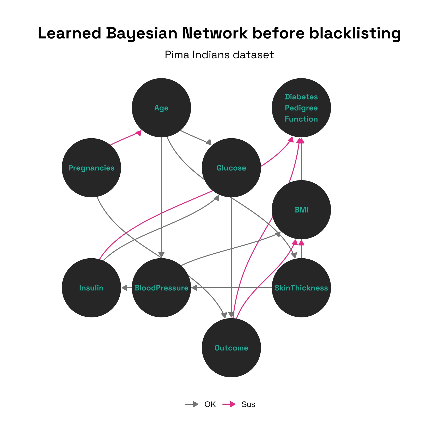
The first thing we should check is if all of the relationships pass the sense check. We can see that several do not, for example: your insulin level, whether you have diabetes, and your BMI do not cause your Diabetes Pedigree Function (a measure of likelihood of diabetes given your family history)1. Further, the outcome (whether you have diabetes) should not cause anything here, since we want to see what causes it.
We can use our prior knowledge to build a blacklist of relationships and then re-run the model:
Blacklisting and visualisation code
blacklist <- tribble(
~from, ~to,
# Pregancies, Age, and Diabetes Pedigree Function are exogenous variables,
# they wouldn't be caused by any of the other variables in the dataset
"Glucose", "Pregnancies",
"Glucose", "Age",
"Glucose", "DiabetesPedigreeFunction",
"BloodPressure", "Pregnancies",
"BloodPressure", "Age",
"BloodPressure", "DiabetesPedigreeFunction",
"SkinThickness", "Pregnancies",
"SkinThickness", "Age",
"SkinThickness", "DiabetesPedigreeFunction",
"Insulin", "Pregnancies",
"Insulin", "Age",
"Insulin", "DiabetesPedigreeFunction",
"BMI", "Pregnancies",
"BMI", "Age",
"BMI", "DiabetesPedigreeFunction",
"Pregnancies", "Age",
# Outcome should not cause anything
"Outcome", "Pregnancies",
"Outcome", "Glucose",
"Outcome", "BloodPressure",
"Outcome", "SkinThickness",
"Outcome", "Insulin",
"Outcome", "BMI",
"Outcome", "DiabetesPedigreeFunction",
"Outcome", "Age",
# Other assumptions
# SkinThickness shouldn't cause BMI
"SkinThickness", "BMI"
)
diabetes_hc_w_blacklist <- hc(diabetes, blacklist = as.matrix(blacklist))
#' Get arc strengths from bnlearn obj
#' NB: This is continuous data, so we use the Gaussian BIC
arc_strengths <- arc.strength(diabetes_hc_w_blacklist, data = diabetes, criterion = "bic-g") %>%
as_tibble()
#' Annotate edges with strength before creating layout
tg_w_bl_annotated <- tg_w_bl %>%
activate(edges) %>%
mutate(
strength = arc_strengths$strength[
match(
paste(.N()$name[from], .N()$name[to]),
paste(arc_strengths$from, arc_strengths$to)
)
]
)
layout_w_bl <- tg_w_bl_annotated %>%
activate(nodes) %>%
left_join(node_positions, by = "name") %>%
create_layout(layout = "manual", x = .$x, y = .$y) %>%
mutate(name = ifelse(name != 'DiabetesPedigreeFunction', name, 'Diabetes\nPedigree\nFunction'))
ggraph(layout_w_bl) +
geom_edge_diagonal(
aes(alpha = abs(strength)),
arrow = arrow(length = unit(2, "mm"), type = 'closed'),
end_cap = circle(12, "mm"),
) +
geom_node_point(size = 30, colour = 'grey20') +
geom_node_text(
aes(label = name),
colour = palette$teal,
family = "space_grotesk",
size = 3,
fontface = "bold"
) +
scale_edge_alpha(range = c(0.2, 1), guide = "none") +
theme_graph() +
theme(
plot.title = element_text(hjust = 0.5, family = "space_grotesk"),
plot.subtitle = element_text(hjust = 0.5, family = "space_grotesk"),
plot.caption = element_text(hjust = 0.5, family = "space_grotesk"),
legend.position = 'none'
) +
coord_cartesian(
xlim = c(-0.67, 4.33),
ylim = c(-0.33, 4.33)
) +
labs(
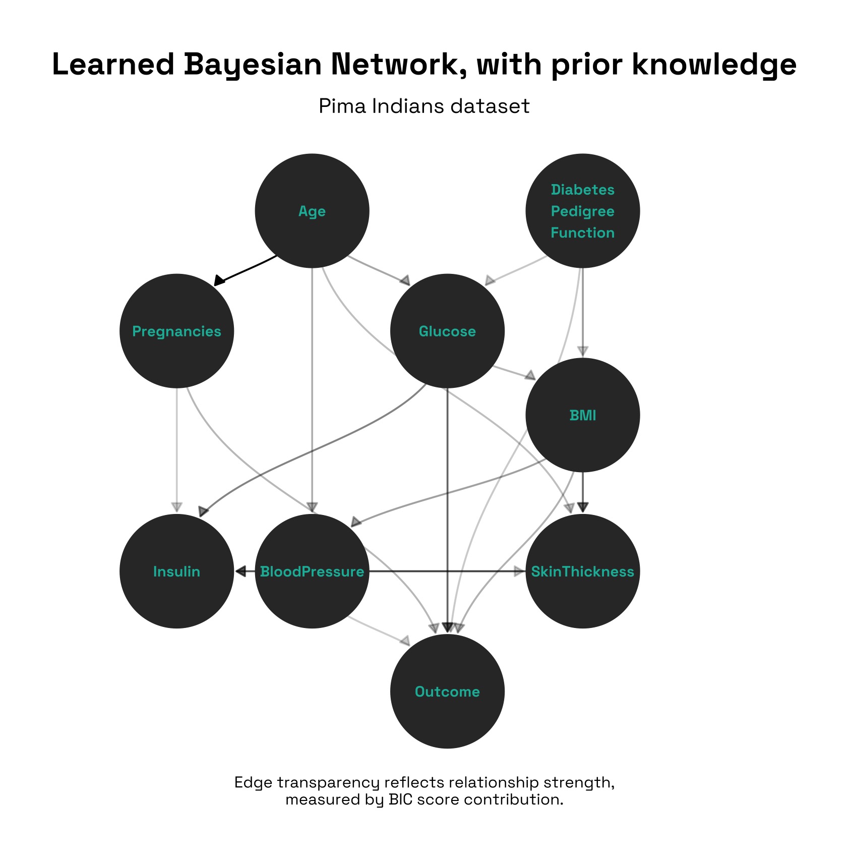
title = 'Learned Bayesian Network, with prior knowledge',
subtitle = 'Pima Indians dataset',
caption = 'Edge transparency reflects relationship strength,\nmeasured by BIC score contribution.'
)
With these constraints in place, we end up with a much more sensible looking graph structure:
The BIC contribution of each relationship is mapped onto the transparency of each edge - where darker edges are stronger BIC contributions, and therefore likely stronger dependencies. For example, the model is fairly certain that the number of pregnancies you’ve had depends on your age, and that your triceps skin fold thickness depends on your BMI.
With the graph structure learnt, we can now move on to calculating the conditional probabilities in the structure with a single call to bnlearn::bn.fit(diabetes_hc_w_blacklist). We can then perform inference over this network - for example, given a patient with glucose above 140, the model estimates their probability of having diabetes at ~60% - which is almost double the unconditional probability of having diabetes in this dataset (~35%).
fitted <- bn.fit(diabetes_hc_w_blacklist, data = diabetes)
cpquery(fitted, event = (Outcome >= 0.5), evidence = (Glucose > 140), n = 1e6)
#> [1] 0.6082396
If we instead learnt the conditional probabilities using a Bayesian method, we could also estimate credible intervals around each inferred probability. However, this takes a bit more effort since we need to specify prior distributions over each conditional probability table.
BNs have lots of powerful applications in real life beyond structure learning, from anomaly detection (scoring how surprising a new observation is under the model) to causal inference (asking not just what correlates to diabetes, but what causes it). Dynamic Bayesian Networks, which extend this framework to model time series, are a topic for a later post.