Introduction
The method
1. The similarity matrix
2. Laplacian matrix
3. Eigendecomposition of the Laplacian
From scratch in R
1. The similarity matrix
2. Laplacian matrix
3. Eigendecomposition of the Laplacian
Limitations

The code for this demo is located here.

Introduction

K-means clustering is a very commonly used tool for unsupervised learning (categorising unlabelled data), however it has its drawbacks. While simple and easy to understand, K-means is biased towards finding spherical clusters (if Euclidean distance is used) or elliptical clusters (if Mahalanobis distance is used). Any non-convex shaped cluster (e.g. a crescent or a spiral) will be misclassified by K-means.

Spectral clustering gets around this by restructuring the clustering problem as a graph problem. Each data point is assigned to a node and relationships between them represent how similar those nodes are. This allows spectral clustering to cluster non-convex shapes as we’ll see later in this post.

This post will discuss how spectral clustering works, while implementing the algorithm from scratch in R.

The method

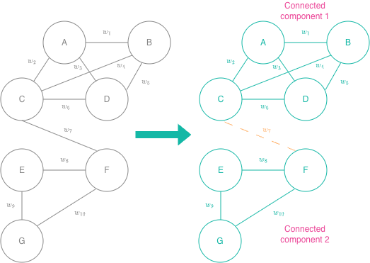
Spectral clustering represents a dataset as an undirected similarity graph that encodes local relationships between observations. Given this similarity graph, clustering becomes a graph partitioning problem where we try to sever the weakest relationships to create isolated but internally well-connected subgraphs which become our clusters.

1. The similarity matrix

We need to represent each observation as a node on the graph, we can do this by constructing a similarity matrix $W$ with similarity measures between each node on the graph. Given a set of $N$ points, we can compute a $N\times N$ matrix of pairwise similarities between all observations.

How can we get the similarity between points? Distance measures such as Euclidean distance get smaller the closer points are but we want a metric that gets larger the closer they are. We can wrap a distance measure in the Gaussian kernel:

s'_{ij}=\exp\big(-\frac{d'_{ij}}{c}\big)

Where $s'_{ij}$ is the similarity between nodes $i$ and $j$ , $d'_{ij}$ is a distance metric such as Euclidean distance, and $c$ is the scale parameter. $exp(-x)$ is a monotonically decreasing function, so smaller values of $x$ yield higher values. We can change the steepness of the kernel by varying $c$ - a smaller $c$ penalises weaker connections more since it keeps the exponent larger, reducing the similarity all else equal.

At this stage, we can draw a graph with $N$ vertices representing the observations and the edges between them weighted with their similarity. In practice, we skip this step and move on to creating the Laplacian matrix.

✂️ Pruning the similarity matrix

While we can use the result of this matrix without any further modification, we can also decide whether to prune weaker connections to keep computation tractable.

If we use the unmodified similarity matrix, we keep all similarity scores. Since all nodes are connected at this stage, $c$ does the heavy lifting in controlling which connections actually matter. $c$ becomes the hyperparameter you tune. We could also use mutual k-nearest neighbours where you only draw an edge between two points if both consider each other a nearest neighbour. Here you’d tune $k$ . We’ll go with this option for this demonstration.

2. Laplacian matrix

Next, we want to create the Laplacian matrix $L$ . This matrix contains the graph structure, as well as how connected each node is to its neighbours. We get this by summing across the rows of the similarity matrix $W$ and putting the results on the diagonal of the degree matrix $G$ :

\begin{aligned} W = \begin{bmatrix} 0 & w_{12} & 0 & 0 & 0 \\ w_{12} & 0 & 0 & w_{24} & 0 \\ 0 & 0 & 0 & w_{34} & 0 \\ 0 & w_{24} & w_{34} & 0 & w_{45} \\ 0 & 0 & 0 & w_{45} & 0 \end{bmatrix} \quad \Rightarrow \quad \begin{aligned} g_1 &= w_{12} \\ g_2 &= w_{12} + w_{24} \\ g_3 &= w_{34} \\ g_4 &= w_{24} + w_{34} + w_{45} \\ g_5 &= w_{45} \end{aligned} \end{aligned}

G = \begin{bmatrix} g_1 & 0 & 0 & 0 & 0 \\ 0 & g_2 & 0 & 0 & 0 \\ 0 & 0 & g_3 & 0 & 0 \\ 0 & 0 & 0 & g_4 & 0 \\ 0 & 0 & 0 & 0 & g_5 \end{bmatrix}

The Laplacian matrix is simply then $L = G - W$ , the degree of how connected each node is less how connected the node is to each of its neighbours. What’s left is a matrix that encodes the connectivity structure of the data, and that measures how much a node differs from its neighbours on average.

3. Eigendecomposition of the Laplacian

The last step is to find the eigenvalues and eigenvectors of the Laplacian. These eigenvectors reveal the directions along which the data are most separable, a smaller eigenvalue indicates a cleaner separation. If we had $m$ perfectly separated clusters in the data, then $L$ would have exactly $m$ zero eigenvalues. However, real data are never perfectly separated, so we look for the $m$ smallest eigenvalues.

Column-binding the $m$ corresponding eigenvectors into a matrix $Z_{N\times m}$ gives us a table where each row of $Z$ is an original observation from the data, represented by its $m$ eigenvector co-ordinates. Projecting the data onto these co-ordinates reveals a data structure that is trivial to cluster, and so we can run K-means on this resulting matrix.

From scratch in R

For this demonstration, we’ll be using the Two Spirals Benchmark Problem from mlbench.

🌀 Data ingestion

set.seed(24601)
spirals_raw <- mlbench::mlbench.spirals(500, cycles = 1, sd = 0.025)

data <- as_tibble(spirals_raw$x, .name_repair = ~c('x', 'y')) %>% 
  mutate(true_label = as.factor(spirals_raw$classes))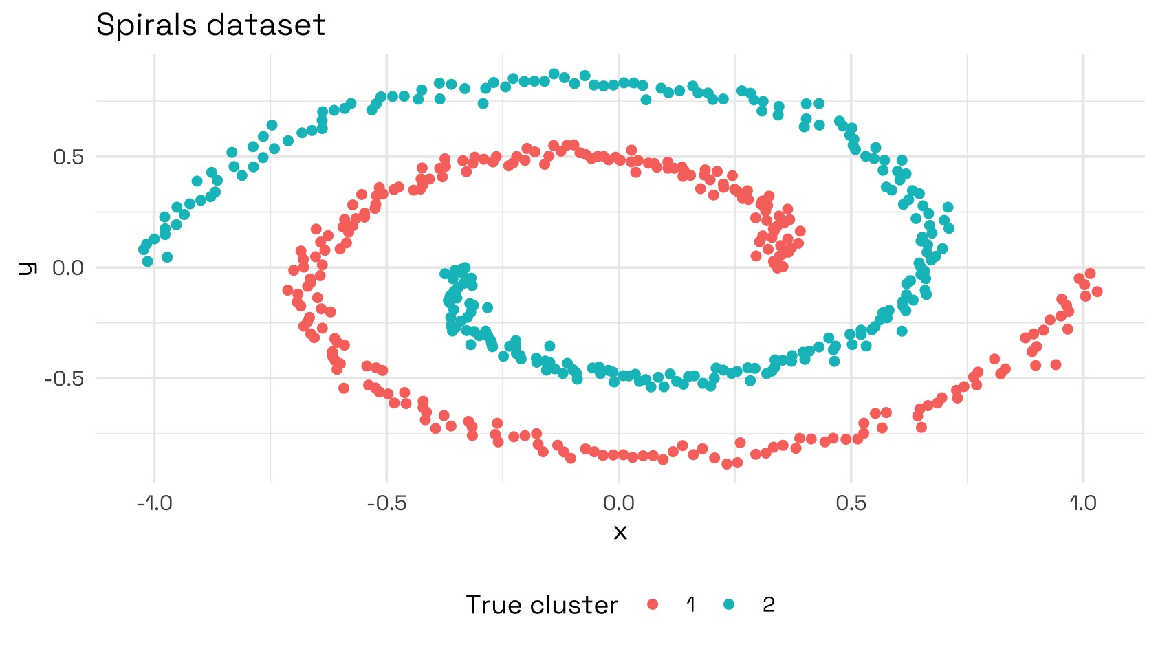

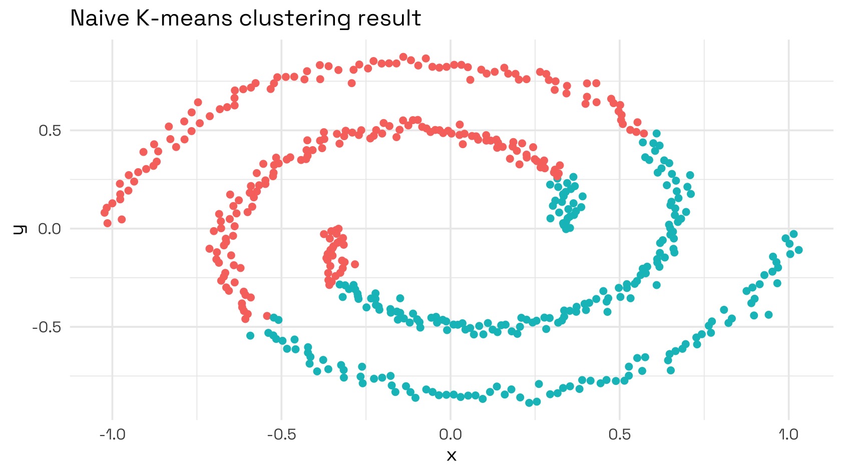
We can see immediately that K-means would fail to classify these groupings accurately:

// K-means clustering fails to accurately discriminate non-convex shaped clusters.

1. The similarity matrix

To build our similarity matrix and then prune it down, we’ll need to pick our $c$ value. For now,a multiple of the median distance between points has been chosen - I’ve picked this using a grid search which I’ll discuss later. Then we’ll use a short function to find the k-th nearest neighbours for each node and filter only for those.

♊ Similarity matrix

c_param <- median(dist(data %>% select(x, y))) * 0.05

make_affinity_matrix <- function(S, k) {

  n  <- nrow(S)
  AM <- matrix(0, nrow = n, ncol = n)

  # For each observation...
  for ( i in seq_len(n) ) {

    # Find the k-th largest similarity scores
    kth_largest <- sort(S[i, ], decreasing = TRUE)[k]

    # and filter out the rest
    neighbours        <- S[i, ] >= kth_largest
    AM[i, neighbours] <- S[i, neighbours]

    # Keep it symmetrical; keep the edge if either 
    # node considers the other a neighbour
    AM[neighbours, i] <- pmax(AM[neighbours, i], S[i, neighbours])

  }

  AM

}

similarity_matrix <- data %>% 
  select(x, y) %>% 
  # Get distance between each pair of points and returns as a 
  # lower triangular matrix
  dist() %>% 
  # Turn this into a full matrix, and mirror both sides of the diagonal
  as.matrix() %>% 
  # Run the Gaussian kernel over all matrix elements
  (function(d, .c_param) exp(-d / .c_param))(c_param)

A <- make_affinity_matrix(similarity_matrix, k = 10)

# Confirm symmetric
all.equal(A, t(A)) # TRUE

Our similarity matrix now looks something like this:

#>      [,1] [,2] [,3] [,4] [,5] 
#> [1,] 1.00 0.00 0.00 0.00 0.00 ...
#> [2,] 0.00 1.00 0.00 0.00 0.74
#> [3,] 0.00 0.00 1.00 0.00 0.00
#> [4,] 0.00 0.00 0.00 1.00 0.00
#> [5,] 0.00 0.74 0.00 0.00 1.00
#>      ...                      ⋱

2. Laplacian matrix

This step is fairly simple, calculate the row sums of the similarity matrix, convert it into a diagonal matrix, then minus the original similarity matrix from it.

⚛️ Laplacian matrix

D <- diag(rowSums(A))
L <- D - A

Our Laplacian looks something like this:

#>      [,1]  [,2] [,3] [,4]  [,5]
#> [1,] 2.37  0.00 0.00 0.00  0.00 ...
#> [2,] 0.00  3.35 0.00 0.00 -0.74
#> [3,] 0.00  0.00 3.39 0.00  0.00
#> [4,] 0.00  0.00 0.00 2.50  0.00
#> [5,] 0.00 -0.74 0.00 0.00  3.47
#>      ...                        ⋱

3. Eigendecomposition of the Laplacian

Finally, we find the eigenvectors and eigenvalues of the Laplacian, find the number of clusters, then take the $m$ smallest eigenvectors. These are then clustered with K-means to get our final cluster assignments.

🔮 Eigendecomposition

eig <- eigen(L)

# Eigenvalues smallest -> largest for readability
eigenvalues <- tibble(
  index = seq_along(eig$values),
  value = rev(eig$values)
)

embedding <- eig$vectors[, (ncol(eig$vectors) - 2 + 1):ncol(eig$vectors)] %>% 
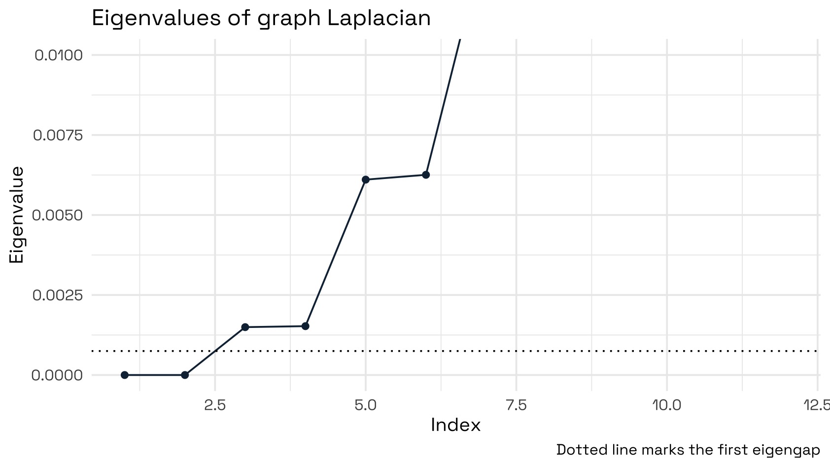
  as_tibble(.name_repair = ~c("z1", "z2"))

We can see clearly that we have two very small eigenvalues before the first clear eigengap that happens between the second smallest and the third smallest eigenvalues. This indicates that our method has picked up on 2 clear cluster groupings.

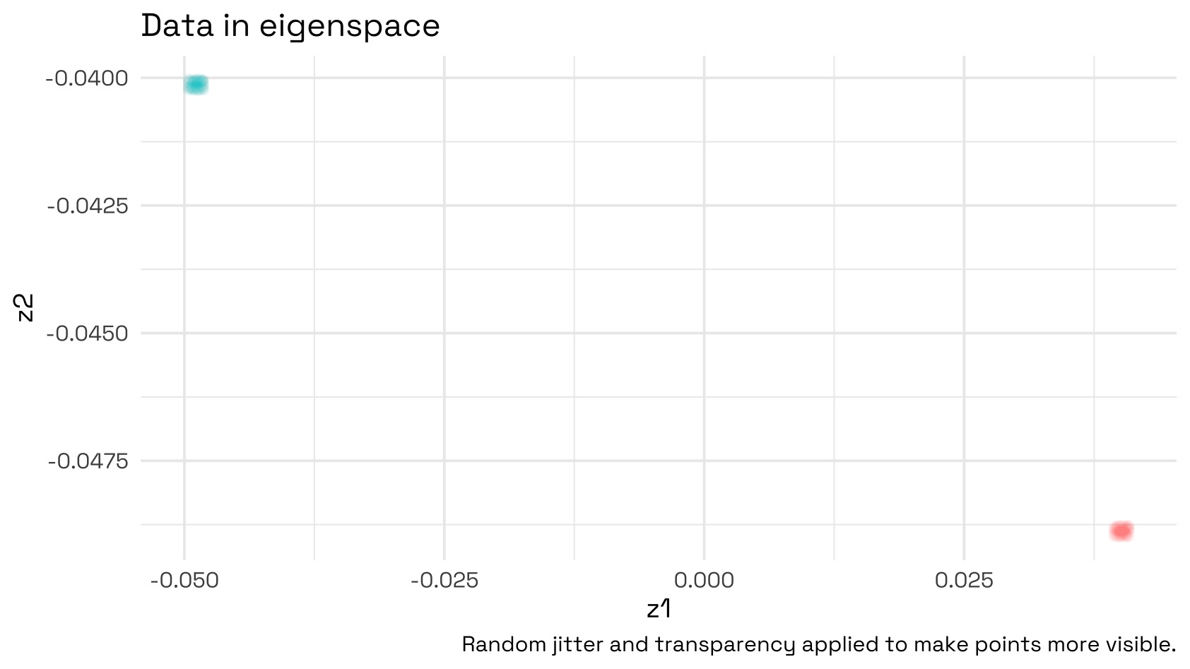
If we then take the two eigenvectors corresponding to those two smallest eigenvalues and plot them, we will see our data projected onto the coordinates of the Laplacian. Notice how the data are now clearly separable and that this is now a trivial task for K-means to properly discriminate between the clusters.

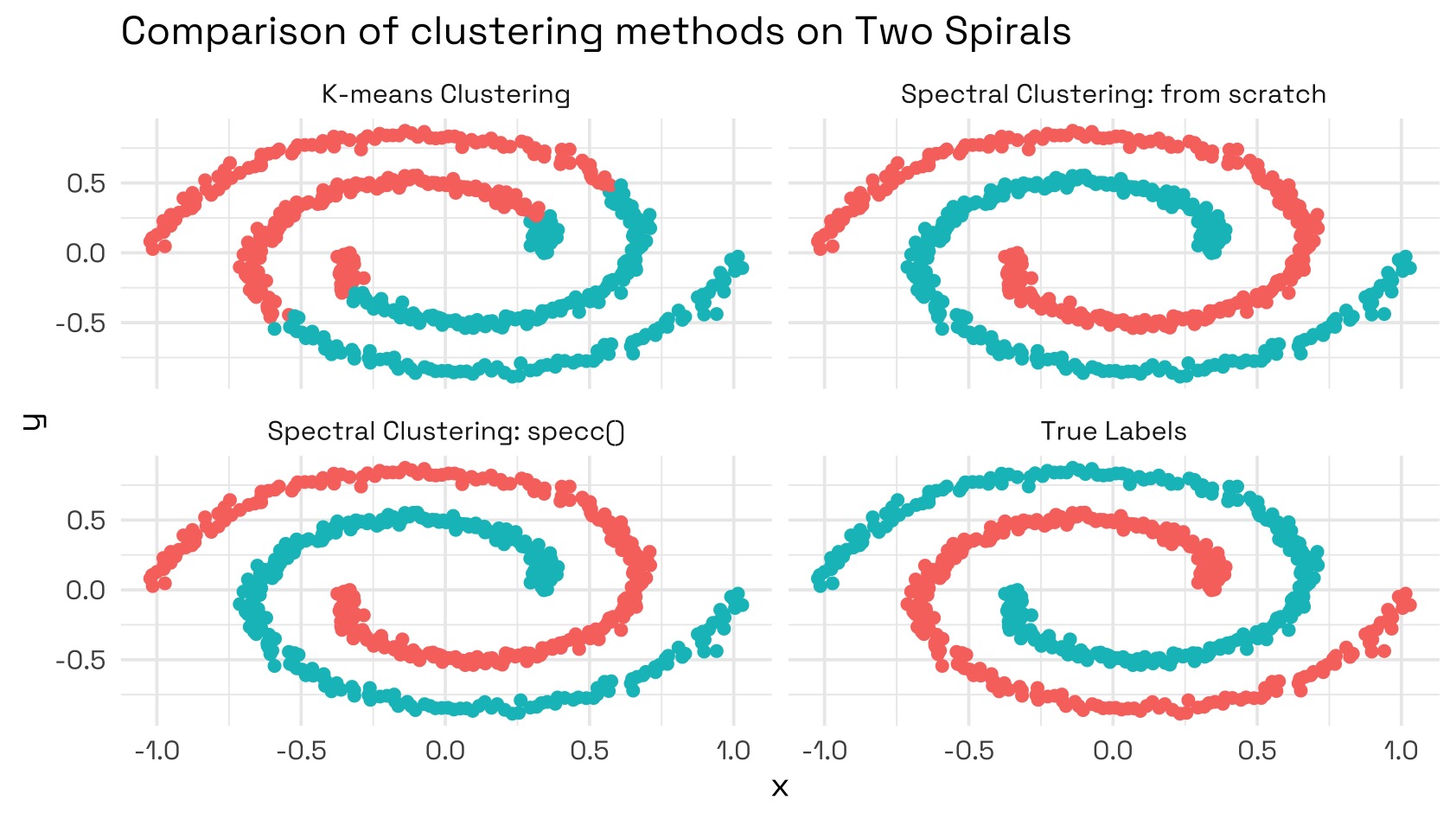
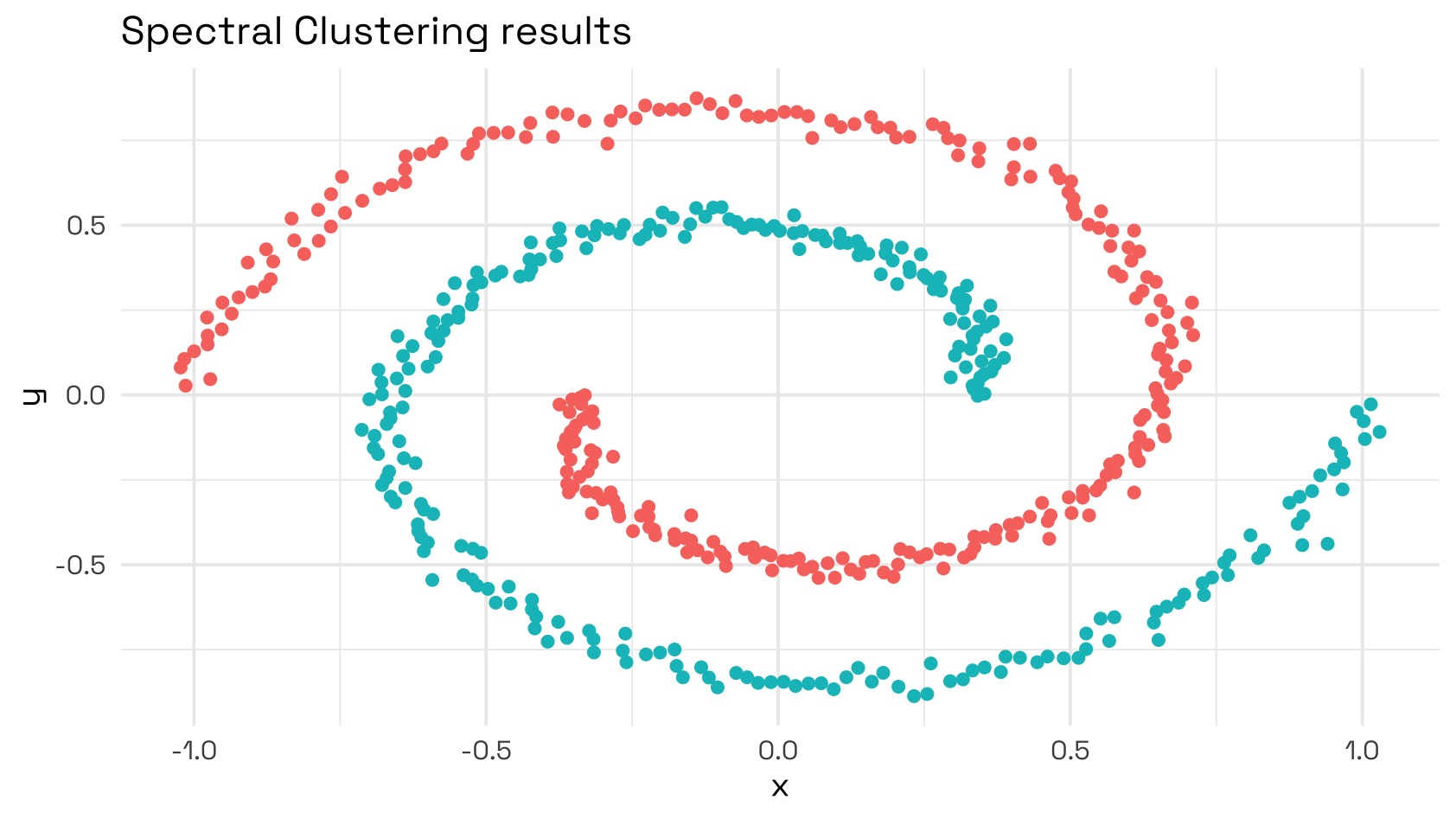
// K-means clustering results shown in blue/red, clusters now trivially separable.

Finally, taking the K-means results from being run over the eigenvector rows and applying them to the original data, we see that spectral clustering works well over this dataset:

Limitations

Despite doing well on this dataset, spectral clustering has its downsides:

This algorithm has a time complexity of $O(n^3)$ , however there are methods that can approximate these results in much faster time.¹
This is not a ‘model’ in that you cannot fit this model to data, then predict over an unseen dataset to assign cluster labels. If you want to give cluster labels to unseen data, you need to run the whole algorithm again.

Finally, arriving at the $c$ and $k$ parameters for this demo required a grid search to achieve a clear eigengap after the second eigenvalue. Had I not known a priori that there were two clusters, I would have been led astray by the eigengap multiple times. Luckily, we don’t need to do this from scratch every time and there are smarter algorithms out there to perform spectral clustering with far less human input:

# No need to manually tune c or k here
specc_model <- kernlab::specc(spirals_raw$x, centers = 2)

Yan, D., Huang, L., & Jordan, M. I. - Fast Approximate Spectral Clustering, UC Berkeley. ↩