• Introduction
• Neural networks
• How backpropagation works
• The loss function
• Gradient descent
• Backpropagation algorithm
• Implementation
• Input data
• Setup
• The main training loop
• Lines 1–4
• Lines 6–16
• Lines 18–33
• Lines 35–47
• Lines 50–55
• Lines >59
• Results

The code for this demonstration may be found here.

Introduction

Inspired by this post by iamtrask, I wanted to create a neural network from scratch with nothing but base (R) language capabilities. The goal here was for me to get a better intuition for how backpropagation updates a neural network’s weights. While my network isn’t quite as terse as iamtrask’s is, I think it’s quite manageable and does a good job at demonstrating how simply we can pull off backprop using linear algebra.

For other sources, I’d highly recommend a read of this blog post: Backprop Explainer, which is great for visual learners and aims to build intuitive understanding. Before we dive into backprop, a quick refresher on neural networks…

Neural networks

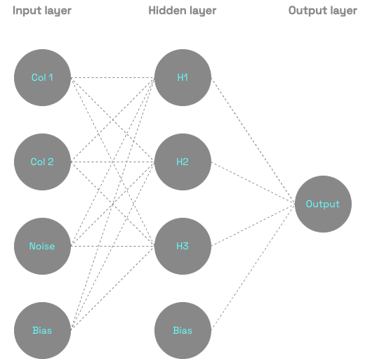
Neural networks at their simplest are a layered arrangement of nodes with three main types: input, hidden, and output. The first layer of nodes captures the input to the network, those inputs are fed into the next layer of hidden nodes, and then on to the output nodes.

Each hidden node is a linear combination of all the values in the previous layer, with coefficients called weights and a possible intercept called a bias. The act of training a neural network is the act of finding the best weights and biases we can. Upon computing this value, it is activated with an activation function. These are how neural networks can learn non-linear shapes, and common activation functions are the sigmoid function, the Rectified Linear Unit (ReLU), or its smooth version, the Gaussian Error Linear Unit (GELU).

In our demonstration, we’ll be using the sigmoid function since it squashes its output to between 0 and 1 which is perfect for us since we’ll be tackling a binary classification task. It’s defined as $\sigma(x)=\frac{1}{1 + e^{-x}}$. Its derivative is also pretty convenient, we can calculate it from the result of the sigmoid: $\sigma'(x)=\sigma(x)(1 - \sigma(x))$.

How backpropagation works

Backpropagation is the algorithm that neural networks use to update their weights, and at its core is the concept of gradient descent. However, before we start, we need to measure how wrong our model is so we know whether we’re improving it or not.

The loss function

To quantify how wrong our model is, we can simply sum our error across all observations in our dataset. Note we square our errors so that positive and negative errors don’t cancel each other out.

Where $\hat{y}_{tk}$ is a function of $\mathbf{w}$ - since the neural network computes $\hat{y}$ by pushing the input through those weights.

As you can imagine, $\mathbf{w}$ is not convex and is instead a complex function with potentially many local minima. We’ll use gradient descent to navigate this function into one of those minima.

Gradient descent

Gradients (i.e. derivatives) tell us how steep a function is at a given point. That means we can use them to figure out which direction we should step in to gain the biggest drop in the loss function. So if we:

• Initialise our weights randomly
• Compute the partial derivatives of our loss function
• Use those to find the direction of the steepest decrease
• Step in that direction, then repeat

We’ll generally reach a local minimum at some point, assuming our steps aren’t so big that we end up stepping back and forth around the actual minimum.

Conveniently, the gradient vector of a function at a given point ($\nabla$) gives us the direction of the largest increase in the function at that point. So to step in the direction of the largest decrease, we step in the direction of $-\nabla$.

Backpropagation makes heavy use of this concept to update the weights of each node.

Backpropagation algorithm

Backpropagation is how a neural network efficiently computes gradients for all weights. The general idea is to:

• Run our inputs through the network so that we can get initial results
• Calculate how wrong those results are, then propagate that error signal backwards through the network, updating weights as we go
• Nodes that contribute the most to the error get updated the most

To get more detailed, at each node, we calculate something along the lines of $\text{error}\times\text{sensitivity}\times\text{activity}=\text{how much value there is in updating this weight}$, where $\text{error}$ is our error signal, $\text{sensitivity}$ tells us how much the output would change if we nudged this weight (it’s the derivative of the node’s activation function), and $\text{activity}$ quantifies how large the input into this node is.

If you’re interested in the calculus:

Let’s get into the implementation.

Implementation

Input data

We’ll be using the example of XOR (exclusive OR) data as our input dataset. This pattern is non-linear, so cannot be learnt by a linear model such as logistic regression - however our neural network will handle it just fine. To our two main input columns, I’ll be adding a bias (a column of 1s, which the network will need to learn XOR), and a white noise column since it’ll be interesting to see how the network minimises the weight of this column by the end of training.

.n_train <- 30
 
# Data ----
# Need to define our input data and target
set.seed(24601)
 
#  2 input cols, our XOR inputs - with an extra random noise column
input_mtx <- cbind(
  sample(c(0, 1), .n_train, replace = TRUE),
  sample(c(0, 1), .n_train, replace = TRUE),
  1, # Bias column, which we can't learn XOR without
  runif(.n_train, -1, 1)
)
 
#  Output is XOR of the first two cols
target_mtx <- xor(input_mtx[, 1], input_mtx[, 2]) |> as.integer()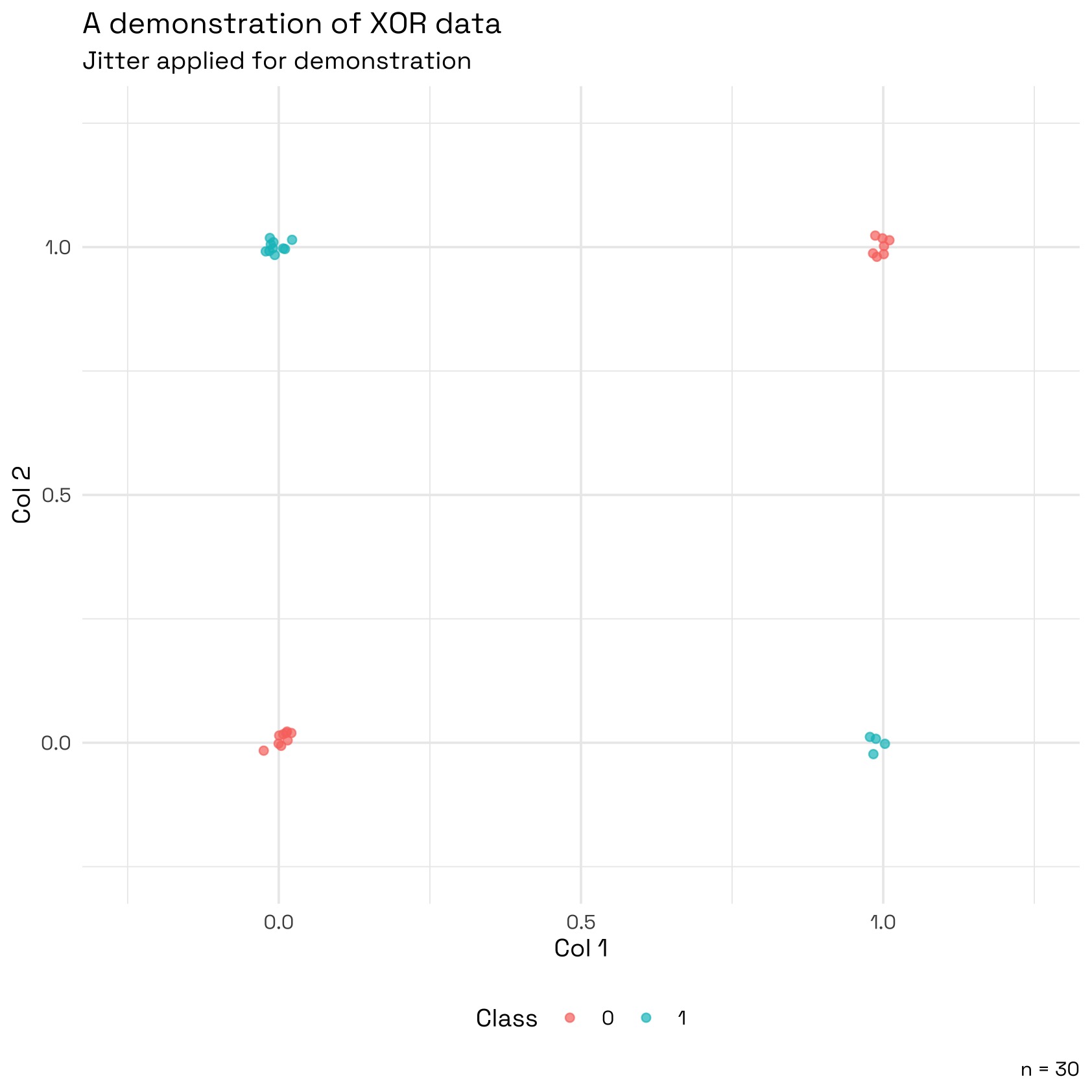

cbind(input_mtx, target_mtx) |> 
  data.frame() |> 
  setNames(c('V1', 'V2', 'Bias', 'Noise', 'Target')) |>
  head()
#>   V1 V2 Bias      Noise Target
#> 1  1  0    1  0.1184642      1
#> 2  1  1    1 -0.1949854      0
#> 3  0  0    1  0.3469756      0
#> 4  0  1    1  0.3771357      1
#> 5  0  0    1 -0.4886959      0
#> 6  0  0    1  0.6804348      0

Setup

I want to set up the dimensions of this neural network so we can use them when defining our weight matrices. Our weight matrices are composed of a column for each node in the layer, and a row for each node in the previous layer. The result at each node within the layer is then the matrix multiplication of the previous layers values and this weight matrix.

These weight matrices actually fully define our neural network, these and the input data are all we need to get started.

nn_dim <- list(layers = 1, nodes_per_layer = 3)
 
init_weights <- function(rows, cols) {
  matrix(runif(rows * cols, -0.5, 0.5), nrow = rows, ncol = cols)
}
 
# 4 nodes in input, so 4 rows. 3 nodes in H1, so 3 cols.
w_ih1 <- init_weights(rows = ncol(input_mtx), cols = nn_dim$nodes_per_layer)
 
# 3 + 1 (bias) nodes in H1, so 4 rows. 1 output, so 1 col.
w_h1o <- init_weights(rows = nn_dim$nodes_per_layer + 1, cols = 1)

We should also define our activation function and its derivative:

# Using a sigmoid/logistic function here. Its derivative uses the result of the
# activation function itself which is computationally convenient.
activation_func <- \(x) 1 / (1 + exp(-x))
activation_func_deriv <- \(x) activation_func(x) * (1 - activation_func(x))

The main training loop

Our training loop for this neural network consists of two passes:

• A forward propagation pass where we push each row of the input data through our neural network, computing weighted sums using the randomly initialised weights.
  • At the end of this, we calculate the loss, i.e. the size of the error.
• A backward propagation pass where we take that loss and pass it backwards through the network, deciding which nodes contributed the most to that error - and therefore which nodes to update the most.

.epochs  <- 1000000
.n_train <- 30
.eta     <- 0.001 # Learning rate
.verbose <- TRUE
 
results <- list()
 
# For each epoch...
for ( epoch in seq_len(.epochs) ) {
  
  if ( .verbose & (epoch %% 1000) == 0 ) message(paste('Epoch:', epoch))
 
  epoch_results <- list(loss = 0)
 
  # ... and each training example ....
  for ( obs in seq_len(nrow(input_mtx)) ) {
 
    ## Forward propagation ----
    # First, perform forward propagation, run the input through the weights and:
    # - Cache the activation function results for use in backpropagation
    # - Record the overall outputs so we know how wrong we are, also for backpropagation
 
    x_i <- matrix(input_mtx[obs, ], nrow = 1)
    y_i <- target_mtx[obs]
 
    # The value at each node is the activated weighted sum of the inputs,
    #  z_1 = input_1 * w_1 + input_2 * w_2 + input_3 * w_3
    z1   <- activation_func(x_i %*% w_ih1)
    z1b  <- cbind(1, z1) # We need a bias node for layer 1 too
    yhat <- activation_func(z1b %*% w_h1o)
 
    # Calculate loss and add it to the overall loss for the epoch
    epoch_results[['loss']] <- epoch_results[['loss']] + (y_i - yhat)^2
 
    ## Backpropagation ----
 
    # This gives us the direction in which to update our weights - i.e. which
    # direction should we step in to yield the largest decrease in loss.
 
    # Output to last hidden layer backprop
    # error * sensitivity * activity = (y - y_hat) * [y_hat * (1 - y_hat)] * z_j
    #                                = (y - y_hat) * activation_func_deriv(y_hat) * z_j
    delta_o <- (y_i - yhat) * activation_func_deriv(yhat)
 
    # First hidden layer to input layer backprop
    delta_h1_full <- activation_func_deriv(z1b) * (delta_o %*% t(w_h1o))
    delta_h1      <- delta_h1_full[, -1, drop = FALSE]   # drop bias column
 
 
    ## Weight updates ----
 
    # w = w + η * δ * activity_of_sending_node
 
    w_h1o <- w_h1o + .eta * (t(z1b) %*% delta_o)
    w_ih1 <- w_ih1 + .eta * (t(x_i) %*% delta_h1)
 
  }
 
  # Assign this epoch's loss back to results list
  # Capture mean absolute weight per input column, alongside loss
  results[[epoch]] <- data.frame(
    epoch        = epoch,
    loss         = 0.5 * epoch_results[['loss']]
  )
 
  if ( .verbose & (epoch %% 1000) == 0 ) cat(paste(' | Loss:', 0.5 * epoch_results[['loss']]), '\n')
 
}
 
loss_df <- do.call(rbind, results)

Let’s walk through this block by block.

Lines 1–4

.epochs  <- 1000000
.eta     <- 0.001 # Learning rate
.verbose <- TRUE

In this block we’re defining a few hyperparameters:

• An epoch is one full pass through the entire training dataset. We’re running 1 million of them here.
• Eta ($\eta$) is the learning rate, i.e. how big are the gradient descent steps we take after each training example is backpropagated through the network
• .verbose is just an internal argument I’m using to decide whether or not to log out epoch numbers whilst training

Lines 6–16

results <- list()
 
# For each epoch...
for ( epoch in seq_len(.epochs) ) {
  
  if ( .verbose & (epoch %% 1000) == 0 ) message(paste('Epoch:', epoch))
 
  epoch_results <- list(loss = 0)
 
  # ... and each training example ....
  for ( obs in seq_len(nrow(input_mtx)) ) {

Here we set up the loop structure of the training process. For each of the 1 million epochs, we run the inner-loop training process for each row of the training data. And to avoid finding ourselves in the R inferno, we define a results list at the start to capture our outputs.

Lines 18–33

   ## Forward propagation ----
    # First, perform forward propagation, run the input through the weights and:
    # - Cache the activation function results for use in backpropagation
    # - Record the overall outputs so we know how wrong we are, also for backpropagation
 
    x_i <- matrix(input_mtx[obs, ], nrow = 1)
    y_i <- target_mtx[obs]
 
    # The value at each node is the activated weighted sum of the inputs,
    #  z_1 = input_1 * w_1 + input_2 * w_2 + input_3 * w_3
    z1   <- activation_func(x_i %*% w_ih1)
    z1b  <- cbind(1, z1) # We need a bias node for layer 1 too
    yhat <- activation_func(z1b %*% w_h1o)
 
    # Calculate loss and add it to the overall loss for the epoch
    epoch_results[['loss']] <- epoch_results[['loss']] + (y_i - yhat)^2

Forward propagation is all about sending our inputs through the neural network with our current weights and biases and getting the outputs out at the end.

• x_i is one row of our training dataset. y_i is the corresponding true class label for that row.
• z1 is a vector of our activated weighted sums, i.e. these are the inputs combined with their weights, biases, and activation function to get the value of the neural net at each node in the first hidden layer. This lends itself well to matrix multiplication:

• z1b is the above vector with a 1 pre-pended to act as our bias node.
• y_hat is the output of pushing our inputs through the network. This is just the values of the first layer of hidden nodes matrix multiplied against the weights from H1 to the output layer, then activated.
• Finally, we add the loss of this training example to the tally for the epoch.

Lines 35–47

   ## Backpropagation ----
 
    # This gives us the direction in which to update our weights - i.e. which
    # direction should we step in to yield the largest decrease in loss.
 
    # Output to last hidden layer backprop
    # error * sensitivity * activity = (y - y_hat) * [y_hat * (1 - y_hat)] * z_j
    #                                = (y - y_hat) * activation_func_deriv(y_hat) * z_j
    delta_o <- (y_i - yhat) * activation_func_deriv(yhat)
 
    # First hidden layer to input layer backprop
    delta_h1_full <- activation_func_deriv(z1b) * (delta_o %*% t(w_h1o))
    delta_h1      <- delta_h1_full[, -1, drop = FALSE]   # drop bias column

Recall that we are trying to minimise $E(w)=\frac{1}{2}\sum^n_{t=1}\sum^K_{k=1}(y_{tk}-\hat{y}_{tk})^2$. Based on gradient descent, our update rule will be $w_i = w_i-\eta\frac{\partial E_t(w)}{\partial w_i}$.

Our equation for that derivative when going from the output node back to the last hidden layer is this: $\frac{\partial E_t(w)}{\partial w^o_{jk}}=-\delta^o_kz_j=-(y_k-\hat{y}_k)\hat{y}_k(1-\hat{y}_k)z_j$ (see the calculus dropdowns above for the derivation).

• delta_o is the error for this training example multiplied by the derivative of the activation function, this is the $(y_k-\hat{y}_k)\hat{y}_k(1-\hat{y}_k)$ part of that equation. Note there’s no leading negative here since that belongs to the full derivative $\frac{\partial E_t(w)}{\partial w^o_{jk}}$, not to $\delta^o_k$ itself. That negative cancels against the one in the gradient descent step.

Given the same error function, our goal is to now update weights between the input and the hidden layer, $w_{ij}^h$. Gradient descent states that our update equation is $w_{ij}^h\leftarrow w^h_{ij}-\eta \frac{\partial E_t(w)}{\partial w_{ij}^h}$. Our equation for that derivative is $\frac{\partial E_t(w)}{\partial w_{ij}^h}=-\delta^h_jx_i=-z_j(1-z_j)x_i\sum^K_{k=1}w_{jk}^o\delta^o_k$.

• $z_j(1-z_j)$ is just the derivative of the sigmoid function at node $j$, which is what we use activation_func_deriv(z1b) for.
• $\sum^K_{k=1}w_{jk}^o\delta^o_k$ gives us the backpropagated error from the outputs - and gives us the error for $j$ based on the extent that it influences wrong outputs via large outgoing weights to outputs with bigger deltas. Here this is done by multiplying the matrix delta_o by the transpose of the weight matrix of H1 to the output: delta_o %*% t(w_h1o).

• $x_i$ is the input to the node. If it is small then adjusting this weight won’t have much effect on the output. We’ll multiply by this in the next step.

Lines 50–55

   ## Weight updates ----
 
    # w = w + η * δ * activity_of_sending_node
 
    w_h1o <- w_h1o + .eta * (t(z1b) %*% delta_o)
    w_ih1 <- w_ih1 + .eta * (t(x_i) %*% delta_h1)

This block finishes computing $\delta^o_k z_j$ and $\delta^h_j x_i$ (the ingredients for our weight update) by multiplying by t(z1b) and t(x_i) respectively. We then multiply by our learning rate .eta and add to the existing weight matrix to complete the weight update. Thats it - backpropagation for this training example is complete!

Lines >59

 # Assign this epoch's loss back to results list
  # Capture mean absolute weight per input column, alongside loss
  results[[epoch]] <- data.frame(
    epoch        = epoch,
    loss         = 0.5 * epoch_results[['loss']]
  )
 
  if ( .verbose & (epoch %% 1000) == 0 ) cat(paste(' | Loss:', 0.5 * epoch_results[['loss']]), '\n')
 
}
 
loss_df <- do.call(rbind, results)

Here we capture a few stats from the training process, the epoch, the total loss from this epoch, and the average weight assigned to each of the input columns.

Results

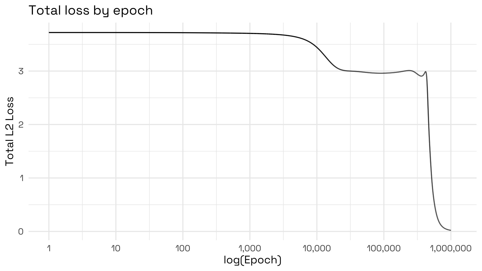
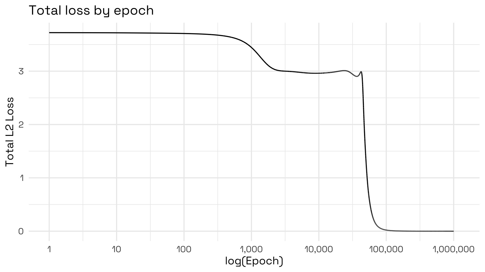
We can watch our loss descend as each epoch passes by plotting those stats we captured. We can see that loss doesn’t actually start dropping significantly until after the 1000th epoch, after which it reaches a plateau then starts to drop drastically, reaching 0 by the 1 millionth epoch. The early plateaus are likely a result of the small and static learning rate; loss improves by a small amount until a breakthrough is reached.

While this works in the end, it’s not efficient: we spend a long time with very little movement. To fix this, we can implement something called momentum. Before we apply the weight update, we blend in a percentage of the previous step’s weight update. This helps the network pick up speed and maintain a downward trend. With this implemented, by epoch 239k we already reach a loss of < 0.001.

# We add a hyperparameter, the percentage of the previous step we blend in
.momentum <- 0.9
 
# Define velocity matrices for momentum implementation
v_h1o <- matrix(0, nrow = nrow(w_h1o), ncol = ncol(w_h1o))
v_ih1 <- matrix(0, nrow = nrow(w_ih1), ncol = ncol(w_ih1))
 
# Then we update our weight change step to output the intermediate raw update,
# apply our momentum to it, then finally update the weight
for (each epoch) {
 
  for (each training sample) {
 
    ...
 
    ## Weight updates ----
 
    # w = w + η * δ * activity_of_sending_node
 
    # This epoch's raw update, before momentum
    grad_h1o <- t(z1b) %*% delta_o
    grad_ih1 <- t(x_i) %*% delta_h1
 
    # Momentum, blend in 90% of the previous weight's update before applying
    v_h1o <- .momentum * v_h1o + grad_h1o
    v_ih1 <- .momentum * v_ih1 + grad_ih1
 
    w_h1o <- w_h1o + .eta * v_h1o
    w_ih1 <- w_ih1 + .eta * v_ih1
 
  }
 
}

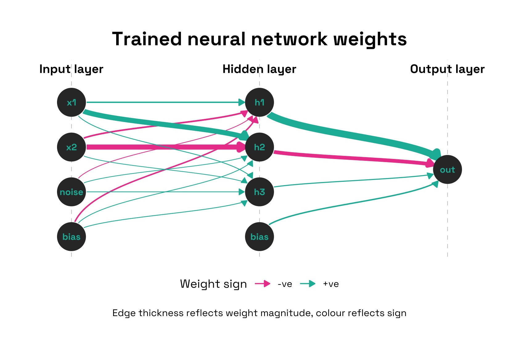
Finally, we can visualise our neural network (using the ggraph and tidygraph packages I used in this previous post). Mapping the magnitude of the weights to the edges, we can see that the network places the most weight on the first and second columns, and barely any weight on the noise column which is what we expected.

As iamtrask’s post mentions, there are plenty of ways we can extend and optimise this implementation (regularisation, dropout, batch normalisation) - but I might leave those for a future post.