Simulating Policy Adoption with Rules-as-Code, DCM and ABM

I have noticed increased interest in predicting or simulating changes in behaviour when policy or software features are introduced: like A/B testing but before anything actually happens. While there is a role for LLM agents to play in simulation, a 2025 critical review of generative social simulation found that of 35 studies surveyed, 22 validated their simulation only by checking whether the output looked believable, not by comparing it against real behaviour. Where researchers did compare rigorously, LLM-generated responses turned out systematically longer, more polite and more articulate than the real human text they were meant to stand in for.

I researched and built a toy policy scenario to validate a robust alternative: a support program meant to help people actually use a new AI tool, calibrated on a real survey dataset, run through a three-layer pipeline that keeps the assumption honest and separable from the evidence.

Rules-as-code decides who's in scope. A discrete choice model estimates one person's probability of adopting. An agent-based model simulates a population of those people, on a network, adopting (or not) over time.

Architecture

Three components, each more complicated if you are new to this space:

1. Rules-as-code (RaC): eligibility as literal data (a JSON-Logic document), evaluated by a small generic rule engine. Not an if buried in application code.
2. Discrete choice model (DCM): a real statistical model of one person's choice, fit on real survey responses. Not a vibe, not an LLM guess.
3. Agent-based model (ABM): a population of agents, resampled from those same respondents, connected on a small-world network, updated over fixed timesteps as adoption spreads.

The toy scenario is calibrated against a real survey of AI adoption at a Vietnamese university, 59 responses scored against UTAUT (Unified Theory of Acceptance and Use of Technology), a widely used model of why people adopt or reject a new technology. UTAUT splits that decision into four factors: performance expectancy (will it help me do my job), effort expectancy (is it easy to use), social influence (do people whose opinion I value think I should use it), and facilitating conditions (do I actually have the support and resources to use it, separate from whether I want to). The toy policy lever targets the last one directly: a facilitating-conditions support program (i.e. invented training/support budget), eligibility gated by role.

Every edge in that diagram maps to a row in an assumption-and-evidence register, covered in Results below.

Implementation

1. Rules-as-code as literal data, not a hardcoded conditional

The eligibility rule is a JSON document, not Python:

{
  "rule": {"==": [{"var": "role"}, "staff"]},
  "note": "Invented toy policy lever for demo purposes only..."
}

A small generic engine evaluates it against whatever facts it's given:

def evaluate_rule(rule: dict, facts: dict) -> bool:
    op, args = next(iter(rule.items()))
 
    def resolve(arg):
        if isinstance(arg, dict) and "var" in arg:
            return facts[arg["var"]]
        return arg
 
    if op == "var":
        return facts[args]
    if op == "in":
        needle, haystack = resolve(args[0]), resolve(args[1])
        return needle in haystack
    if op == "and":
        return all(evaluate_rule(sub, facts) for sub in args)
    if op == "or":
        return any(evaluate_rule(sub, facts) for sub in args)
    if op == "==":
        return resolve(args[0]) == resolve(args[1])
    if op == "!=":
        return resolve(args[0]) != resolve(args[1])
    raise ValueError(f"Unsupported operator: {op}")

Anyone can read or change who's eligible without reading the code that runs it. My original plan gated eligibility on a faculty field that I assumed would exist. The real dataset had no such column, only role, education level, age group and gender. Because the rule is data, that fix was a one-line change to a JSON file, not a code change.

The rule here is hand-written. For what it takes to generate rules-as-code automatically from real legislation instead, see How Executable Is Legislation as Code? An Experiment.

2. A statistical model of one choice, not an LLM roleplaying a population

The DCM is statsmodels logistic regression on four UTAUT constructs, the two-alternative degenerate case of a proper discrete choice model:

FEATURES = ["pe_score", "ee_score", "si_score", "fc_score"]
 
def fit_dcm(df: pd.DataFrame):
    X = sm.add_constant(df[FEATURES])
    y = df["adopter"]
    return sm.Logit(y, X).fit(disp=0, method="bfgs", maxiter=200)

I had to use BFGS (Broyden-Fletcher-Goldfarb-Shanno, a numerical optimisation method that estimates how the likelihood surface curves rather than computing that curvature exactly, the way Newton's method does) instead of the default Newton solver since a 10-row test fixture had two near-perfectly collinear construct scores, and Newton failed to converge on it. BFGS matched Newton's coefficients to four decimal places on every dataset tested and didn't choke on the collinear fixture.

This is a deliberate rejection of the "ask an LLM to be a synthetic citizen" pattern. It's grounded in the same review cited above, not a vibe: most studies never check LLM-simulated behaviour against real behaviour at all. A logistic regression fit on 59 real responses is less exciting to build and more honest about what it actually knows.

3. Turning a lifetime probability into a per-timestep hazard

The DCM gives each agent one number: the probability of having adopted by the end of the run, after all 20 timesteps. The diffusion loop, though, has to decide adoption one timestep at a time. Those are two different quantities, and the gap between them is worth understanding on its own, independent of this project.

If an agent has a lifetime probability p of adopting by the end, and you reuse that same p as the adoption chance at every timestep, the probability of having adopted by timestep T compounds: 1 - (1 - p)^T. That compounds fast. At a 20-step horizon, any agent with a lifetime probability above roughly 15% ends up adopting within the first handful of steps almost for certain, regardless of anything else in the model (this is what tripped me up building the first version of this loop).

Going the other way is the fix: start from the lifetime probability and solve for the per-step hazard that, compounded over all T steps, reproduces it. Given 1 - (1 - hazard)^T = p, rearranging for hazard gives:

step_hazard = 1 - (1 - baseline_prob) ** (1 / self.timesteps)

Each agent gets this per-step hazard once, at construction. The diffusion loop applies step_hazard at every timestep (nudged up or down by peer influence), never the raw lifetime probability. A regression test locks in the closed-form relationship that must hold for every agent, independent of any stochastic draw:

recovered_terminal_prob = 1 - (1 - agent.step_hazard) ** timesteps
assert recovered_terminal_prob == pytest.approx(agent.baseline_prob, abs=1e-9)

This is worth watching for in any model where you calibrate a probability over a lifetime but simulate in discrete steps: survival analysis, churn models, epidemiological SIR (susceptible-infected-recovered) models, anything with an underlying hazard rate. Get it wrong and nothing crashes: no type check catches it, and no unit test that only checks probabilities stay between 0 and 1 will either. It shows up as a headline result that stops responding to the one input it's supposed to be testing.

Results

A full pipeline run produces seven artefacts:

• register (register.csv): every parameter and coefficient the simulation uses, each tagged with how solid it is, observed from real data or expert-assumption
• cohort breakdown (cohort_breakdown.csv): the final adoption rate split by group, staff versus student
• sensitivity tornado chart (sensitivity_tornado.png): how far the final adoption rate swings when each parameter is varied on its own, holding the others fixed
• scenario manifest (scenario_manifest.json): exactly which parameters, seed and dataset version produced this run, so it can be reproduced
• deferral statement (deferral_statement.md): a plain-English statement of what the output can and can't be used for
• causal DAG (causal-dag.md, a directed acyclic graph, i.e. a diagram with no loops): which constructs feed adoption and which parameters govern diffusion, bundled with the run so its assumptions travel with its results
• uncertainty distribution (uncertainty_distribution.csv): the spread of adoption rates across many random seeds, showing how much of the result is genuine signal versus stochastic noise

At a fixed seed (the starting point for the run's random-number generator, pinned so re-running the simulation reproduces byte-identical output instead of a different roll of the dice each time), 300 agents and a 20-step horizon, the eligible cohort (staff) reaches a 58.5% adoption rate; the ineligible cohort (students, who never see the support program) reaches 44.0%. This suggests that the policy had the intended increased adoption effect that we expect.

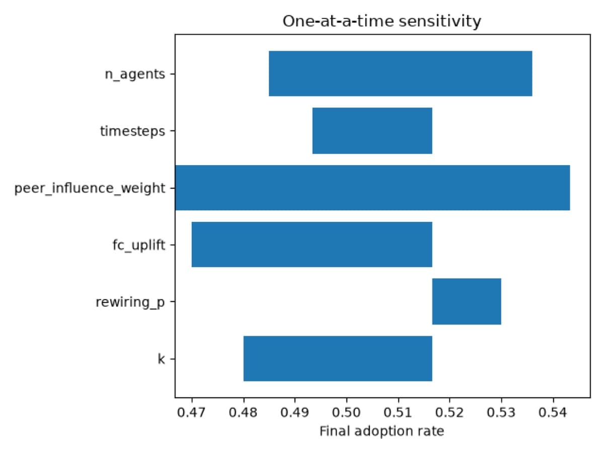
The more useful result is in that chart. Sweeping each ABM parameter one at a time, peer_influence_weight (how strongly an agent is nudged by adopting neighbours) has a wider effect on the final adoption rate than fc_uplift, the actual size of the policy lever. In this calibration, network structure matters more to the outcome than the intervention itself. That's not a result to act on (see the deferral statement below), but it's exactly the kind of quantitative finding a generic adoption curve can't produce.

Every number behind these results is tagged with an evidence strength in register.csv. The DCM's coefficients are tagged observed, fit from real data, with their p-value carried alongside. The ABM's diffusion parameters, network degree, rewiring probability, peer-influence weight, are tagged expert-assumption, because nothing in the source data justifies a specific value for any of them. deferral_statement.md states plainly, next to the results: this is a demo-grade architecture proof of concept, not a validated forecasting tool, and no individual decision should be made or informed by its output.

What Was Hard

Two of the four UTAUT constructs (social influence and facilitating conditions) had no items in the source survey that directly measured them. They're reconstructed from the nearest available item blocks: institutional-readiness and interactivity items standing in for social influence, reverse-coded concern and barrier items standing in for facilitating conditions.

Facilitating conditions is the clearest case of what a proxy costs you. Its raw correlation with the adoption outcome is weakly negative (-0.04), the opposite sign UTAUT theory predicts. Once the other three constructs are controlled for, the fitted DCM coefficient in register.csv flips positive (+0.26), theory-consistent, but nowhere near significant (p = 0.65) at 59 respondents. Both numbers are correct. They answer different questions, and neither one settles whether the proxy is actually measuring facilitating conditions. No amount of code review catches that. It only shows up when someone reads the actual survey questions against the construct they're meant to represent and checks the register for more than its headline sign.

Statistical significance compounds it. Of the four DCM coefficients, only social influence reached conventional significance (p = 0.012). Performance expectancy, effort expectancy and facilitating conditions weren't distinguishable from zero at this sample size. The register's observed tag means "fit from real data." It does not mean "statistically significant." Those are two different claims, and a register that only carries the first one is an easy way to accidentally overstate what a small survey supports.

Where It Goes Next

Retargeting the same pipeline onto a closer-to-real dataset is the obvious next step. The register, DCM and ABM code barely change; the schema-discovery and construct-mapping work, the part that found the proxy-construct limitation above, has to happen again, close to from scratch, against whatever the new dataset's actual columns turn out to be.

If you're the one being asked to put a number on adoption, that's the part worth taking: separate what's observed from what's assumed, tag every number and ship the deferral statement next to the result. The code and the register are both on GitHub below.

Code and Further Reading

Full source is on GitHub. The stack is Python 3.12, pandas, statsmodels, Mesa, NetworkX and matplotlib.

The survey data is pyyjfthc84 on Mendeley Data, a UTAUT-based study of AI adoption at a Vietnamese university.

AI Tools

Claude Code was used to plan and build the demo, including finding and fixing the diffusion-saturation bug during review, and Claude was used to draft this post.