- Published on
- • 14 min read
Running your own LLMs (for beginners)
- Authors

- Name
- Ching Chew
- Socials
To help me prepare for the Hugging Face Fast Gemma Challenge, I took the opportunity to learn how to run LLMs on GPUs. The starting point is to learn the technical terms and concepts so that I can understand what I am researching or experimenting with.
This post is useful if you are asked how much a language model will cost to run, or whether it can run inside your own network at all. Apart from terminology, you will be introduced to levers that you can adjust to improve the performance of LLMs running on your hardware.
The Fast Gemma Challenge rules fix the model, so I could not train anything or swap it for something quicker. The only way through was to learn what each part of the stack actually does. This is that vocabulary, each word attached to the lever it unlocked, plus two measurement mistakes I made along the way. A future post covers how to rent GPUs and serve models outside of the challenge.
The rules
The Fast Gemma Challenge fixes four things: the model (google/gemma-4-E4B-it), the hardware (one A10G GPU), the batch (single stream, one request at a time) and correctness. Everything else is yours to change, including the inference engine (note every number here is on vLLM). Score is tokens per second on 128 held-out prompts.
| Fixed by the rules | What you can change |
|---|---|
| The model and its checkpoint | The inference engine |
| The GPU (one A10G) | Numerics: quantisation, KV-cache dtype |
| Single stream, one request at a time | Execution: compilation, CUDA graphs, attention backend, speculative decoding |
Correctness is a rule too, with two gates: perplexity has to stay under a cap (the reference model scores about 2.30, and the cap is 5 percent above that, about 2.42) and the greedy decode of whatever you submit has to be token-for-token identical to plain greedy decoding of the same checkpoint, with zero tolerance. That second gate is the strict one on paper: it rules out anything that quietly nudges the model's choices, even when the aggregate numbers still look fine.
Because the model is fixed, every lever maps to one concept in the stack around it. That is what makes this a good way to learn the vocabulary.
Checkpoint
A checkpoint is a saved snapshot of a model's trained weights.
This project never trained anything. Every lever either swapped which published checkpoint was loaded or post-processed the weights of one that already existed. When people say "the model" they often mean the architecture plus a specific checkpoint. Here the architecture was locked and the checkpoint nearly so: I could choose among Google's own published variants, including a quantised release, or change individual tensors inside one, but not retrain. Most of what follows is things you can do to a checkpoint without touching how it was trained.
Tokeniser and vocabulary
The tokeniser splits text into short pieces, most of them a few characters long and rarely a whole word. A vocabulary table then maps each piece to an integer ID, and the model only ever works on the IDs. A token is one of those pieces. A single word can be several of them, so token counts never match word counts, which is why pricing is quoted per token.
The tokeniser itself was fixed by the rules. The size of the vocabulary was not incidental, though. Gemma-4's vocabulary has 262,144 entries. The final layer of the model, lm_head, projects the model's internal working vector (its hidden state) to one score per vocabulary entry, so its cost scales with that count. A quarter of a million rows is large enough that a profiler put this one layer at about 25 percent of each decode step.
Quantisation
A model's weights are just numbers, stored by default in 16-bit floating point, sometimes 32-bit. Quantising them means storing them in fewer bits: 8-bit or 4-bit. The model shrinks in memory in proportion: 4-bit weights take a quarter the space of 16-bit ones.
Size is not the point on its own. On a single stream the bottleneck is memory bandwidth. Getting each weight from memory to the compute units takes longer than the arithmetic done with it, so fewer bits per weight means more weights per unit of bandwidth, which means more tokens per second. The cost is precision: round too hard and the model's output changes, which a strict correctness bar will not forgive.
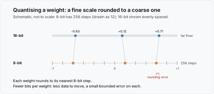
Image 1: a 16-bit float places each weight on a far finer scale than 8-bit's 256 steps. Every weight rounds to its nearest 8-bit step, leaving a small error.
Activations, the intermediate values that flow between layers as the model runs, can be quantised too. The shorthand W8A16 means 8-bit weights and 16-bit activations. Lowering the activation precision as well saves more but is harder to keep accurate, so most recipes quantise the weights only.
Here is what that bought on this model: Google's quantised release left one tensor at full precision: lm_head, the large output projection from the section above. Quantising just that one matrix multiply to 8-bit weights was worth 9.2 percent on real hardware, from 223.62 tokens per second to 244.09. One tensor, one dtype change, a bounded and understandable result.
The whole recipe, in llm-compressor format, is one dict:
# Quantise lm_head, leave every other tensor alone.
{
    "targets": ["re:.*lm_head$"],  # regex, not "lm_head": vLLM nests it as
    "ignore": [],                  # language_model.lm_head under Gemma-4's
    "scheme": "W8A16",             # multimodal wrapper, so an exact-string
    "num_bits": 8,                 # match loads the layer unquantised and
    "type": "int",                 # says nothing
    "symmetric": True,
    "strategy": "channel",
}
That regex-versus-exact-string detail cost an afternoon: the layer loaded, served and stayed at full precision, with no error to say so.
Some key ideas in this space:
QAT (quantisation-aware training) simulates low-precision noise during training so the model learns to tolerate it. PTQ (post-training quantisation) applies it afterwards with no retraining. PTQ is cheaper and riskier, especially against a strict correctness bar.
AWQ and GPTQ are two PTQ methods. AWQ rounds weights to fewer bits, guided by which channels matter most according to calibration data. GPTQ does a more expensive Hessian-based reconstruction. I used AWQ and planned to escalate to GPTQ only if the outputs diverged from the unquantised model.
You can skip that box and still follow the rest. The point that carries over is the worked example: precision is a lever, and you can apply it to a single tensor rather than the entire model.
KV-cache
A model generates one token at a time, and each token it produces is appended to the input for the next step. Ask it for 200 words and it runs the forward pass a couple of hundred times; re-reading the prompt plus everything generated so far on every pass.
Each step, the new token attends to every token before it. The key and value vectors for those earlier tokens do not change from one step to the next, so a naive implementation recomputes the same vectors hundreds of times. The KV-cache stores them after the first pass and hands them back, so each step only computes a key and value for the single new token. It grows with sequence length, and it is often what decides how many requests fit on a GPU at once, which is to say your cost per token.
Two independent levers touched it here. One is the cache's dtype: BF16 against FP8. FP8 halves the memory but is dead on this hardware, because Ampere-class GPUs have no tensor-core support for it, so it was out immediately. The other is sharing: Gemma-4 has a feature where some layers reuse an earlier layer's cache rather than computing their own, which cuts how much cache you carry for the same context.
Attention and head_dim
Attention is the operation where each token looks at the others and decides what to take from them. It runs per head, and each head works in a vector space of a fixed size. That size is head_dim.
Gemma-4 E4B is unusual. Most of its 42 layers use head_dim 256. Seven of them, the global attention layers, use 512. FlashAttention, the fast attention kernel almost everyone reaches for, does not support head_dim 512 on this class of GPU: that path needs kernels gated to newer hardware. The engine saw the mismatch and fell back to a slower kernel. Not only for the 7 incompatible layers. For all 42.
So the default state, before any tuning, is a model running the slow attention path everywhere because seven of its layers cannot use the fast one. That is a large part of why naive serving is slow, and it is invisible unless you go looking for which kernel each layer picked.
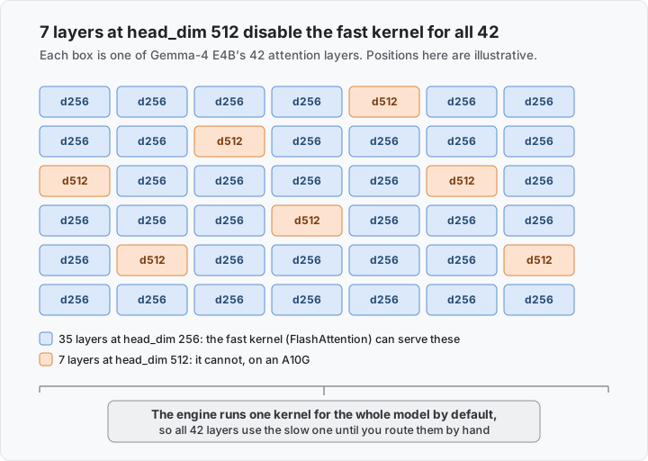
Image 2: seven of the 42 layers use head_dim 512, which the fast kernel cannot serve here. The engine runs one kernel for the whole model by default, so all 42 use the slow path until you route them by hand.
It also explains a reading that catches people out. The GPU sits at 100 percent utilisation from start to finish, which looks like a compute ceiling: the hardware is full, there is nothing more to give. It is not a ceiling. Utilisation means a kernel was scheduled, not that the work it did was the right work. Route the 256-dim layers to the fast kernel and leave the slow one only for the 512-dim global layers, and throughput rises 3.3 percent with the GPU still pegged at 100 percent. The limit was kernel selection, not compute.
The routing is one config object, FlashAttention for the sliding-window (256-dim) layers, Triton for the full-attention (512-dim) ones, passed to vLLM as --attention-config:
{"backend_per_kind": {"sliding_window": "FLASH_ATTN", "full_attention": "TRITON_ATTN"}}Be careful with that 3.3 percent. Fixing the per-layer routing on its own is a real lever and a small one. The full gap to the frontier is a stack of about ten independent patches, not this one change. This is just the change that explains the shape of the problem: the fast path was off for the whole model, and switching it back on where it was allowed bought only a few percent because the rest of the gap lives elsewhere.
The levers that existed but did not decide this
CUDA graphs. A CUDA graph is a recorded, replayable sequence of GPU kernel launches for a fixed shape. It skips the per-step cost of launching each kernel from Python. It matters more here than usual because the batch is one, so each step is small and launch overhead is a larger fraction of it. Worth having, not decisive.
Speculative decoding. A small drafter model proposes several tokens ahead, and the main model verifies them in one batched pass instead of one at a time. K is how many tokens are drafted per step. Acceptance rate is how many the main model agrees with before the first disagreement. A sweep of K across 6, 7 and 8 came out flat, about 236 to 240 tokens per second across all three. The likely reason is the section above: attention was the bottleneck, so drafting more tokens per step just fed more work into the same slow kernel. A lever that does nothing is still information. It told me where the problem was not.
Perplexity and greedy decode
The two correctness gates:
Perplexity measures how surprised the model is by a sequence of tokens, exponentiated, so lower means more confident. The challenge caps it: go as fast as you like, but if perplexity rises more than a few percent above the reference, the run does not count.
Greedy decode is the other gate. Decoding greedily means taking the single highest-scoring token at each step, with no sampling. Your submission's greedy output has to match plain greedy decoding of the same checkpoint exactly.
Here is the mistake. For weeks my local perplexity probe was wrong, and wrong in the flattering direction. It measured the model's confidence in tokens the model had chosen itself. That is close to circular: a model is always fairly confident in its own greedy picks. The real scoring harness measures perplexity against a fixed reference sequence the model never generated. Every number the probe gave me was biased low. The sharpest case was the frontier reproduction: scored the right way, its real margin against the cap was about half a percent, where my local number had implied plenty of room.
Greedy-identical had its own surprise. My submission fails it at token 4, and the cause is not quantisation corrupting a confident decision. It is a genuine tie in the unquantised model's own logits, where two tokens score close enough that a trivial numerical difference flips which one wins. The automated scoring never actually re-checks greedy-identical, so the submission was scored regardless. Still worth knowing before you trust a zero-tolerance gate: some of what it would catch is the model being genuinely undecided, not you breaking it.
What this bought
The naive baseline was about 223 tokens per second. My best submission was about 244. The reproduced frontier was about 526. The one lever I shipped was lm_head quantisation, worth 9.2 percent, which is the whole distance from 223 to 244. A second lever, per-layer attention routing, measured at another 3.3 percent, but I left it out of the submission.
The rest of the way to 526 is the field's shared toolkit, ported between competitors' entries: depth pruning that drops 5 of the 42 layers, 4-bit weights, a fine-tuned drafter, a trimmed output vocabulary, one CUDA graph over the whole verify loop and a fast detokenise path. About ten independent patches, none of them a single trick, and reproducing them is a project in itself.
K tuning, the lever that felt like it should matter most, contributed nothing.
One more measurement note, because it cost me a day. On a development GPU, not the competition's A10G, I re-ran an unchanged config twice and got 635 then 943 tokens per second. Nothing changed between runs except the GPU's boost clock ramping and a compiler cache warming up. The absolute numbers are high because it is a faster card in a looser test, but the point is the 1.5x swing between two identical runs. That looks exactly like a real lever effect. The rule I use now: any throughput comparison needs at least three restarts with the launch order rotated, or the first-run numbers will lie to you.
Next time a deck puts a tokens-per-second figure in front of you, ask which checkpoint it ran, which attention backend, how many restarts sit behind the number and what hardware produced it.
Code and Further Reading
- The Fast Gemma Challenge: huggingface.co/gemma-challenge
- My competition code: github.com/cchew/gemma-challenge (MIT)
- vLLM: docs.vllm.ai. Quantisation recipes: llm-compressor
- FlashAttention: github.com/Dao-AILab/flash-attention
- AWQ: arxiv.org/abs/2306.00978. GPTQ: arxiv.org/abs/2210.17323
- Speculative decoding: arxiv.org/abs/2211.17192
- Perplexity for fixed-length models: huggingface.co/docs/transformers/en/perplexity
- See a transformer run one token, step by step: Brendan Bycroft's LLM Visualization
AI Tools
Claude Code was used to run and document the competition experiments, and Claude was used to draft this post from those notes.